TECHNIQUES FOR
TECHNIQUES FOR
NOISE ROBUSTNESS IN
AUTOMATIC SPEECH
RECOGNITION
Editors
Tuomas Virtanen
Tampere University of Technology, Finland
Rita Singh
Carnegie Mellon University, USA
Bhiksha Raj
Carnegie Mellon University, USA
Registered office
John Wiley & Sons Ltd, The Atrium, Southern Gate, Chichester, West Sussex, PO19 8SQ, United Kingdom For details of our global editorial offices, for customer services and for information about how to apply for permission to reuse the copyright material in this book please see our website at www.wiley.com.
The right of the author to be identified as the author of this work has been asserted in accordance with the Copyright, Designs and Patents Act 1988.
All rights reserved. No part of this publication may be reproduced, stored in a retrieval system, or transmitted, in any form or by any means, electronic, mechanical, photocopying, recording or otherwise, except as permitted by the UK Copyright, Designs and Patents Act 1988, without the prior permission of the publisher.
Wiley also publishes its books in a variety of electronic formats. Some content that appears in print may not be available in electronic books.
Designations used by companies to distinguish their products are often claimed as trademarks. All brand names and product names used in this book are trade names, service marks, trademarks or registered trademarks of their respective owners. The publisher is not associated with any product or vendor mentioned in this book. This publication is designed to provide accurate and authoritative information in regard to the subject matter covered. It is sold on the understanding that the publisher is not engaged in rendering professional services. If professional advice or other expert assistance is required, the services of a competent professional should be sought.
Library of Congress Cataloging-in-Publication Data Virtanen, Tuomas.
Techniques for noise robustness in automatic speech recognition / Tuomas Virtanen, Rita Singh, Bhiksha Raj. p. cm.
Includes bibliographical references and index. ISBN 978-1-119-97088-0 (cloth)
1. Automatic speech recognition. I. Singh, Rita. II. Raj, Bhiksha. III. Title. TK7882.S65V57 2012
006.4′54–dc23
2012015742 A catalogue record for this book is available from the British Library.
ISBN: 978-0-470-97409-4
List of Contributors xv
Acknowledgments xvii
1 Introduction 1
Tuomas Virtanen, Rita Singh, Bhiksha Raj
1.1 Scope of the Book 1
1.2 Outline 2
1.3 Notation 4
Part One FOUNDATIONS
2 The Basics of Automatic Speech Recognition 9
Rita Singh, Bhiksha Raj, Tuomas Virtanen
2.1 Introduction 9
2.2 Speech Recognition Viewed as Bayes Classification 10
2.3 Hidden Markov Models 11
2.3.1 Computing Probabilities with HMMs 12
2.3.2 Determining the State Sequence 17
2.3.3 Learning HMM Parameters 19
2.3.4 Additional Issues Relating to Speech Recognition Systems 20
2.4 HMM-Based Speech Recognition 24
2.4.1 Representing the Signal 24
2.4.2 The HMM for a Word Sequence 25
2.4.3 Searching through all Word Sequences 26
References 29
3 The Problem of Robustness in Automatic Speech Recognition 31 Bhiksha Raj, Tuomas Virtanen, Rita Singh
3.1 Errors in Bayes Classification 31
3.1.1 Type 1 Condition: Mismatch Error 33
3.1.2 Type 2 Condition: Increased Bayes Error 34
3.2 Bayes Classification and ASR 35
3.2.2 Intrinsic Interferences—Signal Components that are Unrelated to
the Message: A Type 2 Condition 36
3.2.3 External Interferences—The Data are Noisy: Type 1 and
Type 2 Conditions 36
3.3 External Influences on Speech Recordings 36
3.3.1 Signal Capture 37
3.3.2 Additive Corruptions 41
3.3.3 Reverberation 42
3.3.4 A Simplified Model of Signal Capture 43
3.4 The Effect of External Influences on Recognition 44
3.5 Improving Recognition under Adverse Conditions 46
3.5.1 Handling the Model Mismatch Error 46
3.5.2 Dealing with Intrinsic Variations in the Data 47
3.5.3 Dealing with Extrinsic Variations 47
References 50
Part Two SIGNAL ENHANCEMENT
4 Voice Activity Detection, Noise Estimation, and Adaptive Filters for
Acoustic Signal Enhancement 53
Rainer Martin, Dorothea Kolossa
4.1 Introduction 53
4.2 Signal Analysis and Synthesis 55
4.2.1 DFT-Based Analysis Synthesis with Perfect Reconstruction 55 4.2.2 Probability Distributions for Speech and Noise DFT Coefficients 57
4.3 Voice Activity Detection 58
4.3.1 VAD Design Principles 58
4.3.2 Evaluation of VAD Performance 62
4.3.3 Evaluation in the Context of ASR 62
4.4 Noise Power Spectrum Estimation 65
4.4.1 Smoothing Techniques 65
4.4.2 Histogram and GMM Noise Estimation Methods 67
4.4.3 Minimum Statistics Noise Power Estimation 67
4.4.4 MMSE Noise Power Estimation 68
4.4.5 Estimation of theA PrioriSignal-to-Noise Ratio 69
4.5 Adaptive Filters for Signal Enhancement 71
4.5.1 Spectral Subtraction 71
4.5.2 Nonlinear Spectral Subtraction 73
4.5.3 Wiener Filtering 74
4.5.4 The ETSI Advanced Front End 75
4.5.5 Nonlinear MMSE Estimators 75
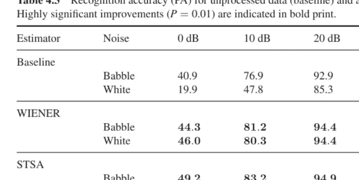
4.6 ASR Performance 80
4.7 Conclusions 81
5 Extraction of Speech from Mixture Signals 87 Paris Smaragdis
5.1 The Problem with Mixtures 87
5.2 Multichannel Mixtures 88
5.2.1 Basic Problem Formulation 88
5.2.2 Convolutive Mixtures 92
5.3 Single-Channel Mixtures 98
5.3.1 Problem Formulation 98
5.3.2 Learning Sound Models 100
5.3.3 Separation by Spectrogram Factorization 101
5.3.4 Dealing with Unknown Sounds 105
5.4 Variations and Extensions 107
5.5 Conclusions 107
References 107
6 Microphone Arrays 109
John McDonough, Kenichi Kumatani
6.1 Speaker Tracking 110
6.2 Conventional Microphone Arrays 113
6.3 Conventional Adaptive Beamforming Algorithms 120
6.3.1 Minimum Variance Distortionless Response Beamformer 120
6.3.2 Noise Field Models 122
6.3.3 Subband Analysis and Synthesis 123
6.3.4 Beamforming Performance Criteria 126
6.3.5 Generalized Sidelobe Canceller Implementation 129
6.3.6 Recursive Implementation of the GSC 130
6.3.7 Other Conventional GSC Beamformers 131
6.3.8 Beamforming based on Higher Order Statistics 132
6.3.9 Online Implementation 136
6.3.10 Speech-Recognition Experiments 140
6.4 Spherical Microphone Arrays 142
6.5 Spherical Adaptive Algorithms 148
6.6 Comparative Studies 149
6.7 Comparison of Linear and Spherical Arrays for DSR 152
6.8 Conclusions and Further Reading 154
References 155
Part Three FEATURE ENHANCEMENT
7 From Signals to Speech Features by Digital Signal Processing 161 Matthias W¨olfel
7.1 Introduction 161
7.1.1 About this Chapter 162
7.3 Spectral Processing 163
7.3.1 Windowing 163
7.3.2 Power Spectrum 165
7.3.3 Spectral Envelopes 166
7.3.4 LP Envelope 166
7.3.5 MVDR Envelope 169
7.3.6 Warping the Frequency Axis 171
7.3.7 Warped LP Envelope 175
7.3.8 Warped MVDR Envelope 176
7.3.9 Comparison of Spectral Estimates 177
7.3.10 The Spectrogram 179
7.4 Cepstral Processing 179
7.4.1 Definition and Calculation of Cepstral Coefficients 180
7.4.2 Characteristics of Cepstral Sequences 181
7.5 Influence of Distortions on Different Speech Features 182
7.5.1 Objective Functions 182
7.5.2 Robustness against Noise 185
7.5.3 Robustness against Echo and Reverberation 187
7.5.4 Robustness against Changes in Fundamental Frequency 189
7.6 Summary and Further Reading 191
References 191
8 Features Based on Auditory Physiology and Perception 193
Richard M. Stern, Nelson Morgan
8.1 Introduction 193
8.2 Some Attributes of Auditory Physiology and Perception 194
8.2.1 Peripheral Processing 194
8.2.2 Processing at more Central Levels 200
8.2.3 Psychoacoustical Correlates of Physiological Observations 202 8.2.4 The Impact of Auditory Processing on Conventional
Feature Extraction 206
8.2.5 Summary 208
8.3 “Classic” Auditory Representations 208
8.4 Current Trends in Auditory Feature Analysis 213
8.5 Summary 221
Acknowledgments 222
References 222
9 Feature Compensation 229
Jasha Droppo
9.1 Life in an Ideal World 229
9.1.1 Noise Robustness Tasks 229
9.1.2 Probabilistic Feature Enhancement 230
9.2 MMSE-SPLICE 232
9.2.1 Parameter Estimation 233
9.2.2 Results 236
9.3 Discriminative SPLICE 237
9.3.1 The MMI Objective Function 238
9.3.2 Training the Front-End Parameters 239
9.3.3 The Rprop Algorithm 240
9.3.4 Results 241
9.4 Model-Based Feature Enhancement 242
9.4.1 The Additive Noise-Mixing Equation 243
9.4.2 The Joint Probability Model 244
9.4.3 Vector Taylor Series Approximation 246
9.4.4 Estimating Clean Speech 247
9.4.5 Results 247
9.5 Switching Linear Dynamic System 248
9.6 Conclusion 249
References 249
10 Reverberant Speech Recognition 251
Reinhold Haeb-Umbach, Alexander Krueger
10.1 Introduction 251
10.2 The Effect of Reverberation 252
10.2.1 What is Reverberation? 252
10.2.2 The Relationship between Clean and Reverberant
Speech Features 254
10.2.3 The Effect of Reverberation on ASR Performance 258
10.3 Approaches to Reverberant Speech Recognition 258
10.3.1 Signal-Based Techniques 259
10.3.2 Front-End Techniques 260
10.3.3 Back-End Techniques 262
10.3.4 Concluding Remarks 265
10.4 Feature Domain Model of the Acoustic Impulse Response 265
10.5 Bayesian Feature Enhancement 267
10.5.1 Basic Approach 268
10.5.2 Measurement Update 269
10.5.3 Time Update 270
10.5.4 Inference 271
10.6 Experimental Results 272
10.6.1 Databases 272
10.6.2 Overview of the Tested Methods 273
10.6.3 Recognition Results on Reverberant Speech 274
10.6.4 Recognition Results on Noisy Reverberant Speech 276
10.7 Conclusions 277
Acknowledgment 278
Part Four MODEL ENHANCEMENT
11 Adaptation and Discriminative Training of Acoustic Models 285 Yannick Est`eve, Paul Del´eglise
11.1 Introduction 285
11.1.1 Acoustic Models 286
11.1.2 Maximum Likelihood Estimation 287
11.2 Acoustic Model Adaptation and Noise Robustness 288
11.2.1 Static (or Offline) Adaptation 289
11.2.2 Dynamic (or Online) Adaptation 289
11.3 MaximumA PosterioriReestimation 290
11.4 Maximum Likelihood Linear Regression 293
11.4.1 Class Regression Tree 294
11.4.2 Constrained Maximum Likelihood Linear Regression 297
11.4.3 CMLLR Implementation 297
11.4.4 Speaker Adaptive Training 298
11.5 Discriminative Training 299
11.5.1 MMI Discriminative Training Criterion 301
11.5.2 MPE Discriminative Training Criterion 302
11.5.3 I-smoothing 303
11.5.4 MPE Implementation 304
11.6 Conclusion 307
References 308
12 Factorial Models for Noise Robust Speech Recognition 311
John R. Hershey, Steven J. Rennie, Jonathan Le Roux
12.1 Introduction 311
12.2 The Model-Based Approach 313
12.3 Signal Feature Domains 314
12.4 Interaction Models 317
12.4.1 Exact Interaction Model 318
12.4.2 Max Model 320
12.4.3 Log-Sum Model 321
12.4.4 Mel Interaction Model 321
12.5 Inference Methods 322
12.5.1 Max Model Inference 322
12.5.2 Parallel Model Combination 324
12.5.3 Vector Taylor Series Approaches 326
12.5.4 SNR-Dependent Approaches 331
12.6 Efficient Likelihood Evaluation in Factorial Models 332
12.6.1 Efficient Inference using the Max Model 332
12.6.2 Efficient Vector-Taylor Series Approaches 334
12.6.3 Band Quantization 335
12.7 Current Directions 337
12.7.2 Multi-Talker Speech Recognition using Graphical Models 339 12.7.3 Noise Robust ASR using Non-Negative
Basis Representations 340
References 341
13 Acoustic Model Training for Robust Speech Recognition 347 Michael L. Seltzer
13.1 Introduction 347
13.2 Traditional Training Methods for Robust Speech Recognition 348
13.3 A Brief Overview of Speaker Adaptive Training 349
13.4 Feature-Space Noise Adaptive Training 351
13.4.1 Experiments using fNAT 352
13.5 Model-Space Noise Adaptive Training 353
13.6 Noise Adaptive Training using VTS Adaptation 355
13.6.1 Vector Taylor Series HMM Adaptation 355
13.6.2 Updating the Acoustic Model Parameters 357
13.6.3 Updating the Environmental Parameters 360
13.6.4 Implementation Details 360
13.6.5 Experiments using NAT 361
13.7 Discussion 364
13.7.1 Comparison of Training Algorithms 364
13.7.2 Comparison to Speaker Adaptive Training 364
13.7.3 Related Adaptive Training Methods 365
13.8 Conclusion 366
References 366
Part Five COMPENSATION FOR INFORMATION LOSS
14 Missing-Data Techniques: Recognition with Incomplete Spectrograms 371 Jon Barker
14.1 Introduction 371
14.2 Classification with Incomplete Data 373
14.2.1 A Simple Missing Data Scenario 374
14.2.2 Missing Data Theory 376
14.2.3 Validity of the MAR Assumption 378
14.2.4 Marginalising Acoustic Models 379
14.3 Energetic Masking 381
14.3.1 The Max Approximation 381
14.3.2 Bounded Marginalisation 382
14.3.3 Missing Data ASR in the Cepstral Domain 384
14.3.4 Missing Data ASR with Dynamic Features 386
14.4 Meta-Missing Data: Dealing with Mask Uncertainty 388
14.4.2 Sub-band Combination Approaches 391
14.4.3 Speech Fragment Decoding 393
14.5 Some Perspectives on Performance 395
References 396
15 Missing-Data Techniques: Feature Reconstruction 399
Jort Florent Gemmeke, Ulpu Remes
15.1 Introduction 399
15.2 Missing-Data Techniques 401
15.3 Correlation-Based Imputation 402
15.3.1 Fundamentals 402
15.3.2 Implementation 404
15.4 Cluster-Based Imputation 406
15.4.1 Fundamentals 406
15.4.2 Implementation 408
15.4.3 Advances 409
15.5 Class-Conditioned Imputation 411
15.5.1 Fundamentals 411
15.5.2 Implementation 412
15.5.3 Advances 413
15.6 Sparse Imputation 414
15.6.1 Fundamentals 414
15.6.2 Implementation 416
15.6.3 Advances 418
15.7 Other Feature-Reconstruction Methods 420
15.7.1 Parametric Approaches 420
15.7.2 Nonparametric Approaches 421
15.8 Experimental Results 421
15.8.1 Feature-Reconstruction Methods 422
15.8.2 Comparison with Other Methods 424
15.8.3 Advances 426
15.8.4 Combination with Other Methods 427
15.9 Discussion and Conclusion 428
Acknowledgments 429
References 430
16 Computational Auditory Scene Analysis and Automatic
Speech Recognition 433
Arun Narayanan, DeLiang Wang
16.1 Introduction 433
16.2 Auditory Scene Analysis 434
16.3 Computational Auditory Scene Analysis 435
16.3.1 Ideal Binary Mask 435
16.4 CASA Strategies 440
16.4.1 IBM Estimation Based on Local SNR Estimates 440
16.4.2 IBM Estimation using ASA Cues 442
16.4.3 IBM Estimation as Binary Classification 448
16.4.4 Binaural Mask Estimation Strategies 451
16.5 Integrating CASA with ASR 452
16.5.1 Uncertainty Transform Model 454
16.6 Concluding Remarks 458
Acknowledgment 458
References 458
17 Uncertainty Decoding 463
Hank Liao
17.1 Introduction 463
17.2 Observation Uncertainty 465
17.3 Uncertainty Decoding 466
17.4 Feature-Based Uncertainty Decoding 468
17.4.1 SPLICE with Uncertainty 470
17.4.2 Front-End Joint Uncertainty Decoding 471
17.4.3 Issues with Feature-Based Uncertainty Decoding 472
17.5 Model-Based Joint Uncertainty Decoding 473
17.5.1 Parameter Estimation 475
17.5.2 Comparisons with Other Methods 476
17.6 Noisy CMLLR 477
17.7 Uncertainty and Adaptive Training 480
17.7.1 Gradient-Based Methods 481
17.7.2 Factor Analysis Approaches 482
17.8 In Combination with Other Techniques 483
17.9 Conclusions 484
References 485
Jon Barker
University of Sheffield, UK Paul Del´eglise
University of Le Mans, France Jasha Droppo
Microsoft Research, USA Yannick Est`eve
University of Le Mans, France Jort Florent Gemmeke KU Leuven, Belgium Reinhold Haeb-Umbach
University of Paderborn, Germany John R. Hershey
Mitsubishi Electric Research Laboratories, USA Dorothea Kolossa
Ruhr-Universit¨at Bochum, Germany Alexander Krueger
University of Paderborn, Germany Kenichi Kumatani
Disney Research, USA Jonathan Le Roux
Hank Liao Google Inc., USA Rainer Martin
Ruhr-Universit¨at Bochum, Germany John McDonough
Carnegie Mellon University, USA Nelson Morgan
International Computer Science Institute and the University of California, Berkeley, USA Arun Narayanan
The Ohio State University, USA Bhiksha Raj
Carnegie Mellon University, USA Ulpu Remes
Aalto University School of Science, Finland Steven J. Rennie
IBM Thomas J. Watson Research Center, USA Michael L. Seltzer
Microsoft Research, USA Rita Singh
Carnegie Mellon University, USA Paris Smaragdis
University of Illinois at Urbana-Champaign, USA Richard Stern
Carnegie Mellon University, USA Tuomas Virtanen
Tampere University of Technology, Finland DeLiang Wang
The Ohio State University, USA Matthias W¨olfel
The editors would like to thank Jort Gemmeke, Joonas Nikunen, Pasi Pertil¨a, Janne Pylkk¨onen, Ulpu Remes, Rahim Saeidi, Michael Wohlmayr, Elina Helander, Kalle Palom¨aki, and Katariina Mahkonen, who have have assisted by providing constructive comments about individual chapters of the book.
1
Introduction
Tuomas Virtanen
1, Rita Singh
2, Bhiksha Raj
21
Tampere University of Technology, Finland 2Carnegie Mellon University, USA
1.1
Scope of the Book
The term “computer speech recognition” conjures up visions of the science-fiction capabil-ities of HAL2000 in2001, A Space Odessey, or “Data,” the anthropoid robot inStar Trek, who can communicate through speech with as much ease as a human being. However, our real-life encounters with automatic speech recognition are usually rather less impressive, com-prising often-annoying exchanges with interactive voice response, dictation, and transcription systems that make many mistakes, frequently misrecognizing what is spoken in a way that humans rarely would. The reasons for these mistakes are many. Some of the reasons have to do with fundamental limitations of the mathematical framework employed, and inadequate awareness or representation of context, world knowledge, and language. But other equally important sources of error are distortions introduced into the recorded audio during recording, transmission, and storage.
As automatic speech-recognition—or ASR—systems find increasing use in everyday life, the speech they must recognize is being recorded over a wider variety of conditions than ever before. It may be recorded over a variety ofchannels, including landline and cellular phones, the internet, etc. using different kinds of microphones, which may be placed close to the mouth such as in head-mounted microphones or telephone handsets, or at a distance from the speaker, such as desktop microphones. It may be corrupted by a wide variety ofnoises, such as sounds from various devices in the vicinity of the speaker, general background sounds such as those in a moving car or background babble in crowded places, or even competing speakers. It may also be affected byreverberation, caused by sound reflections in the recording environment. And, of course, all of the above may occur concurrently in myriad combinations and, just to make matters more interesting, may change unpredictably over time.
Techniques for Noise Robustness in Automatic Speech Recognition, First Edition. Edited by Tuomas Virtanen, Rita Singh, and Bhiksha Raj.
For speech-recognition systems to perform acceptably, they must berobustto the distorting influences. This book deals with techniques that impart such robustness to ASR systems. We present a collection of articles from experts in the field, which describe an array of strategies that operate at various stages of processing in an ASR system. They range from techniques for minimizing the effect of external noises at the point of signal capture, to methods of deriving features from the signal that are fundamentally robust to signal degradation, techniques for attenuating the effect of external noises on the signal, and methods for modifying the recognition system itself to recognize degraded speech better.
The selection of techniques described in this book is intended to cover the range of ap-proaches that are currently considered state of the art. Many of these apap-proaches continue to evolve, nevertheless we believe that for a practitioner of the field to follow these developments, he must be familiar with the fundamental principles involved. The articles in this book are designed and edited to adequately present these fundamental principles. They are intended to be easy to understand, and sufficiently tutorial for the reader to be able to implement the described techniques.
1.2
Outline
Robustnesss techniques for ASR fall into a number of different categories. This book is divided into five parts, each focusing on a specific category of approaches. A clear understanding of robustness techniques for ASR requires a clear understanding of the principles behind automatic speech recognition and the robustness issues that affect them. These foundations are briefly discussed in Part One of the book. Chapter 2 gives a short introduction to the fundamentals of automatic speech recognition. Chapter 3 describes various distortions that affect speech signals, and analyzes their effect on ASR.
Part Two discusses techniques that are aimed at minimizing the distortions in the speech signal itself.
Chapter 4 presents methods forvoice-activity detection(VAD),noise estimation, and noise-suppressiontechniques based on filtering. A VAD analyzes which signal segments correspond to speech and which to noise, so that an ASR system does not mistakenly interpret noise as speech. VAD can also provide an estimate of the noise during periods of speech inactivity. The chapter also reviews methods that are able to track noise characteristics even during speech activity. Noise estimates are required by many other techniques presented in the book.
Chapter 5 presents two approaches for separating speech from noises. The first one uses multiple microphones and an assumption that speech and noise signals are statistically inde-pendent of each other. The method does not usea prioriinformation about the source signals, and is therefore termedblind source separation. Statistically independent signals are separated using an algorithm calledindependent component analysis. The second approach requires only a single microphone, but it is based ona prioriinformation about speech or noise signals. The presented method is based on factoring the spectrogram of noisy speech into speech and noise usingnonnegative matrix factorization.
speech source. The chapter first presents the fundamentals of conventional linear microphone arrays, then reviews different criteria that can be used to design them, and then presents methods that can be used in the case ofspherical microphone arrays.
Part Three of the book discusses methods that attempt to minimize the effect of distortions onacoustic featuresthat are used to represent the speech signal.
Chapter 7 reviews conventional feature extraction methods that typically parameterize the envelope of the spectrum. Both methods based onlinear predictionandcepstralprocessing are covered. The chapter then discussesminimum variance distortionless responseorwarping techniques that can be applied to make the envelope estimates more reliable for purposes of speech recognition. The chapter also studies the effect of distortions on the features.
Chapter 8 approaches the noise robustness problem from the point of view of human speech perception. It first presents a series of auditory measurements that illustrate selected properties of the human auditory system, and then discusses principles that make the human auditory system less sensitive to external influences. Finally, it presents several computationalauditory modelsthat mimic human auditory processes to extract noise robust features from the speech signal.
Chapter 9 presents methods that reduce the effect of distortions on features derived from speech. Thesefeature-enhancementtechniques can be trained to map noisy features to clean ones using training examples of clean and noisy speech. The mapping can include a criterion which makes the enhanced features morediscriminative, i.e., makes them more effective for speech recognition. The chapter also presents methods that use an explicit model for additive noises.
Chapter 10 focuses on the recognition of reverberant speech. It first analyzes the effect of reverberation on speech and the features derived from it. It gives a review of different approaches that can be used to perform recognition of reverberant speech and presents methods for enhancing features derived from reverberant speech based on a model of reverberation.
Part Four discusses methods which modify the statistical parameters employed by the recognizer to improve recognition of corrupted speech.
Chapter 11 presents adaptation methods which change the parameters of the recognizer without assuming a specific kind of distortion. Thesemodel-adaptation techniques are fre-quently used to adapt a recognizer to a specific speaker, but can equally effectively be used to adapt it to distorted signals. The chapter also presents training criteria that makes the statistical models in the recognizer morediscriminative, to improve the recognition performance that can be obtained with them.
Chapter 12 focuses on compensating for the effect of interfering sound sources on the recognizer. Based on a model of interfering noises and a model of the interaction process between speech and noise, these model-compensation techniques can be used to derive a statistical model for noisy speech. In order to find a mapping between the models for clean and noisy speech, the techniques use various approximations of the interaction process.
Chapter 13 discusses a methodology that can be used to find the parameters of an ASR system to make it more robust, given any signal or feature enhancement method. These noise-adaptive-trainingtechniques are applied in the training stage, where the parameters the ASR system are tuned to optimize the recognition accuracy.
Chapter 14 first discusses the general taxonomy of different missing-data problems. It then discusses the conditions under which speech features can be considered reliable, and when they may be assumed to be missing. Finally, it presents methods that can be used to perform robust ASR when there is uncertainty about which parts of the signal are missing.
Chapter 15 presents methods that produce an estimate of missing features (i.e., feature reconstruction) using reliable features. Reconstruction methods based on a Gaussian mixture model utilize local correlations between missing and reliable features. The reconstruction can also be done separately for each state of the ASR system. Sparse representation methods model the noisy observation as a linear combination of a small number of atomic units taken from a larger dictionary, and the weights of the atomic units are determined using reliable features only.
Chapter 16 discusses methods that estimate which parts of a speech signal are missing and which ones are reliable. The estimation can be based either on the signal-to-noise ratio in each time-frequency component, or on more perceptually motivated cues derived from the signal, or using a binary classification approach.
Chapter 17 presents approaches which enable the modeling of theuncertaintycaused by noise in the recognition system. It first discusses feature-based uncertainty, which enables modeling of the uncertainty in enhanced signals or features obtained through algorithms discussed in the previous chapters of the book. Model-based uncertainty decoding, on the other hand, enables us to account for uncertainties in model compensation or adaptation techniques. The chapter also discusses the use of uncertainties with noise-adaptive training techniques.
We also revisit the contents of the book in the end of Chapter 3, once we have analyzed the types of errors encountered in automatic speech recognition.
1.3
Notation
The table below lists the most commonly used symbols in the book. Some of the chapters deviate from the definitions below, but in such cases the used symbols are explicitly defined.
Symbol Definition
a, b, c, . . . Scalar variables
A, B, C, . . . Constants a,b,c, . . . Vectors A,B,C, . . . Matrices
⊗ Convolution
N Normal distribution
E{x} Expected value ofx
AT Transpose of matrixA
xi:j Setxi, xi+ 1, . . . , xj
s Speech signal
n Additive noise signal
x Noisy speech signal
h Response from speaker to microphone
Symbol Definition
f Frequency index
xt Observation vector of noisy speech in framet
q State variable
qt State at timet
µ Mean vector
Θ,Σ Covariance matrix
2
The Basics of Automatic
Speech Recognition
Rita Singh
1, Bhiksha Raj
1, Tuomas Virtanen
21
Carnegie Mellon University, USA 2
Tampere University of Technology, Finland
2.1
Introduction
In order to understand the techniques described later in this book, it is important to understand how automatic speech-recognition (ASR) systems function. This chapter briefly outlines the framework employed by ASR systems based on hidden Markov models (HMMs).
Most mainstream ASR systems are designed as probabilistic Bayes classifiers that identify the most likely word sequence that explains a given recorded acoustic signal. To do so, they use an estimate of the probabilities of possible word sequences in the language, and the probability distributions of the acoustic signals for each word sequence. Both the probability distributions of word sequences, and those of the acoustic signals for any word sequence, are represented through parametricmodels. Probabilities of word sequences are modeled by various forms of grammars orN-gram models. The probabilities of the acoustic signals are modeled by HMMs. In the rest of this chapter, we will briefly describe the components and process of ASR as outlined above, as a prelude to explaining the circumstances under which it may perform poorly, and how that relates to the remaining chapters of this book. Since this book primarily addresses factors that affect theacousticsignal, we will only pay cursory attention to the manner in which word-sequence probabilities are modeled, and elaborate mainly on the modeling of the acoustic signal.
In Section 2.2, we outline Bayes classification, as applied to speech recognition. The fundamentals of HMMs—how to calculate probabilities with them, how to find the most likely explanation for an observation, and how to estimate their parameters—are given in Section 2.3. Section 2.4 describes how HMMs are used in practical ASR systems. Several issues related to practical implementation are addressed. Recognition is not performed with
Techniques for Noise Robustness in Automatic Speech Recognition, First Edition. Edited by Tuomas Virtanen, Rita Singh, and Bhiksha Raj.
the speech signal itself, but onfeaturesderived from it. We give a brief review of the most commonly used features in Section 2.4.1. Feature computation is covered in greater detail in Chapters 7 and 8 of the book. The number of possible word sequences that must be investigated in order to determine the most likely one is potentially extremely large. It is infeasible to explicitly characterize the probability distributions of the acoustics for each and every word sequence. In Sections 2.4.2 and 2.4.3, we explain how we can nevertheless explore all of them bycomposingthe HMMs for word sequences from smaller units, and how the set of all possible word sequences can be represented as compact graphs that can be searched.
Before proceeding, we note that although this book largely presents speech recognition and robustness issues related to it from the perspective of HMM-based systems, the fundamental ideas presented here, and many of the algorithms and techniques described both in this chapter and elsewhere in the book, carry over to other formalisms that may be employed for speech recognition as well.
2.2
Speech Recognition Viewed as Bayes Classification
At their core, state-of-art ASR systems are fundamentallyBayesian classifiers. The Bayesian classification paradigm follows a rather simple intuition: the best guess for the explanation of any observation (such as a recording of speech) is the mostlikely one, given any other information we have about the problem at hand. Mathematically, it can be stated as follows: let C1,C2, C3, . . . represent all possible explanations for an observationX. The Bayesian classification paradigm chooses the explanationCisuch that
P(Ci|X, θ)≥P(Cj|X, θ) ∀j=i, (2.1)
where P(Ci|X, θ)is the conditional probability of class Ci given the observationX, andθ represents all other evidence, or information knowna priori. In other words, it chooses the a posteriorimost probable explanationCi, given the observation and all prior evidence.
For theASRproblem, the problem is now stated as follows. Given a speech recordingX, the sequence of wordswˆ1,wˆ2,· · ·that were spoken is estimated as
ˆ
w1,w2ˆ ,· · ·= argmax w1,w2,···
P(w1, w2,· · · |X,Λ). (2.2)
Here,Λrepresents other evidence that we may have about what was spoken. Equation (2.2) states that the “best guess” word sequencewˆ1,wˆ2· · ·is the word sequence that isa posteriori most probable, after consideration of both the recordingXand all other evidence represented byΛ.
In order to implement Equation (2.2) computationally, the problem is refactored using Bayes’ rule as follows:
ˆ
w1,w2,ˆ · · ·= argmax w1,w2,···
P(X|w1, w2,· · ·)P(w1, w2,· · · |Λ). (2.3)
The second term on the right-hand side of Equation (2.3),P(w1, w2,· · · |Λ), provides the a prioriprobability of a word sequence, given all other evidenceΛ. In theory,Λmay include evidence from our knowledge of the linguistic structure of the language (i.e., how people usually string words together when they speak), about the context of the current conversation, world knowledge, and anything else that one might bring to bear on the problem. However, in practice, the probability of a word sequence is usually assumed to be completely specified by alanguage model. The language model is often represented as afinite-stateor acontext-free grammar, or alternatively, as a statisticalN-grammodel.
2.3
Hidden Markov Models
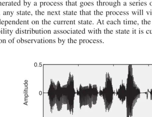
Speech signals aretime-seriesdata, i.e., they are characterized by a sequence of measurements x0,x1,· · ·, where the sequence represents a progression through time andxt represents the tth measurement in the series (the exact nature of the measurementxtis discussed in Section 2.4.1). In the case of speech, this time series isnonstationary, i.e., its characteristics vary with time, as illustrated by the example in Figure 2.1.
HMMs are statistical models of time-series data. An HMM models a time series as having been generated by a process that goes through a series ofstatesfollowing a Markov chain. When in any state, the next state that the process will visit is determined stochastically and is only dependent on the current state. At each time, the process draws an observation from a probability distribution associated with the state it is currently in. Figure 2.2 illustrates the generation of observations by the process.
0 0.5 1 1.5 2
–0.5 0 0.5
Time (s)
Time (s)
Amplitude
Frequency (Hz)
0.5 1 1.5 2
0 2000 4000 6000 8000
State sequence
Observation sequence
Figure 2.2 Left panel: schematic illustration of an HMM. The four circles represent the states of the HMM and the arrows represent allowed transitions. Each HMM state is associated with a state output distribution as shown. Right panel: generation of an observation sequence. The process progresses thorough a sequence of states. At each visited state, it generates an observation by drawing from the corresponding state output distribution.
Mathematically, an HMM is described as a probabilistic function of a Markov chain [11], and is adoubly stochasticmodel. The first level of this model is a Markov chain that is specified by aninitialstate probability distribution, usually denoted asπ, and a transition matrix, which we will denote as A.π specifies the probability of finding the process in any state at the very first instant. Representing the sequence of states visited by the process as q0, q1,· · ·, π(i) =P(q0 =i)is the probability that at the very first instant the process will be in statei. Ais a matrix whose(i, j)th entryai,j =P(qt+ 1=j|qt=i)represents the probability that the process will transitionto state j, given that the process is currently in statei. The Markov chain thus is a probabilistic specification of the manner in which the process progresses through states.
The second level of the model is a set ofstate outputprobability distributions, one associated with each state. We denote the state output probability distribution associated with any statei asP(x|i), or more succinctly asPi(x). If the process arrives at stateiat timet, it generates an observationxtby drawing it from the state output distributionPi(x).
When HMMs are employed in speech-recognition systems the state output distributions are usually modeled as Gaussian mixture densities, andPi(x)has the form
Pi(x) = K
k= 1
wi,kN(x;µi,k,Θi,k), (2.4)
whereN(x;µ,Θ)represents a multivariate Gaussian density with mean vectorµand covari-ance matrixΘ.wi,k,µi,kandΘi,kare the mixture weight, mean vector, and covariance matrix of thekth Gaussian in the mixture Gaussian state output distribution for statei.Kis the number of Gaussians in the mixture.
2.3.1
Computing Probabilities with HMMs
Having defined the parameters of an HMM, we now explain how various probabilities can be computed from them.
The Probability of Following a Specific State Sequence
sequenceq0:T−1=q0, q1,· · ·, qT−1can be written using Bayes’ rule as
P(q0:T−1) =P(q0)P(q1|q0)P(q2|q0, q1)· · ·P(qT−1|q0· · ·qT−2) = P(q0)P(q1|q0)P(q2|q1)· · ·P(qT−1|qT−2)
= P(q0) T−1
t= 1
P(qt|qt−1) (2.5)
= πq0 T−1
t= 1
aqt−1,qt.
Here, we have used the Markovian property of the process: at any time, the future behavior of the process depends only on the current state and not on how it arrived there. Thus, P(qt|q0· · ·qt−1) =P(qt|qt−1).
The Probability of Generating a Specific Observation Sequence from a Given State Sequence
We can also compute the probability that the process will produce a specific observation sequence x0:T−1 =x0,x1,· · ·,xT−1, when it follows a specific state sequence q0:T−1 = q0, q1,· · ·, qT−1. According to the model, the observation generated by the process at any time depends only on the state that the process is currently in, that isP(xt|q0, q1,· · ·, qT−1) = P(xt|qt) =Pqt(xt). Thus,
P(x0:T−1|q0:T−1) = T−1
t= 0
Pqt(xt). (2.6)
The Probability of Following a Particular State Sequence and Generating a Specific Observation Sequence
The joint probability of following a particular state sequence and generating a specific ob-servation sequence can be factored into two terms: the product of a probability of a state sequence (2.5) and a state-sequence conditional probability of an observation sequence (2.6), as illustrated in Figure 2.3. The probability that the process will proceed through a par-ticular state sequence q0:T−1 and generate an observation sequence x0:T−1 can thus be stated as
P(x0:T−1, q0:T−1) =P(x0:T−1|q0:T−1)P(q0:T−1)
=P(q0)P(x0|q0) T−1
t= 1
P(qt|qt−1)P(xt|qt) (2.7)
=πq0Pq0(x0) T−1
t= 1
State sequence
State sequence
Observation sequence
Figure 2.3 An HMM process can be factored into two parts: following a state sequence (top panel) and generating the observation sequence from the state sequence (bottom panel).
The Forward Probability
The probabilityP(x0:t, qt=i)that the process arrives at stateiat timetwhile generating the firsttobservationsx0:t, is often called theforwardprobability and denoted byα(i, t). Att= 0, when there have been no transitions, we only need to consider the initial state of the process and the first observation, and therefore
α(i,0) =P(x0, q0 =i)
=P(x0|q0 =i)P(q0=i) =Pq0(x0)πq0.
Thereafter,α(i, t)can be recursively defined. In order to arrive at statejat timet, the process must be at some stateiatt−1and transition toj. Thus, the probability that the process will follow a state sequence that takes it through iatt−1 and arrive atjat tand generate the observation sequencex0:t =x0:t−1,xtis merely the probability that the process will arrive at iatt−1while generatingx0:t−1, transition fromitojand finally generatextfromj, that is
P(x0:t, qt−1 =i, qt=j) =P(x0:t−1, qt−1 =i)P(qt=j|qt−1 =i)P(xt|qt=j) =α(i, t−1)ai,jPj(xt).
Since α(j, t)is not a function of the state att−1,i must be integrated out from the above equation:
α(j, t) = Q
i= 1
P(x0:t, qt−1 =i, qt=j) (2.9)
=Pj(xt) Q
i= 1
α(i, t−1)ai,j, (2.10)
j,t
Time xt
State index
x0
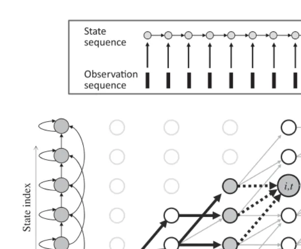
Figure 2.4 A “Trellis” showing all possible state sequences that the HMM on the left may follow to generate the observation sequence shown at the bottom. The thick solid lines show the “forward” subtrellis representing all state sequences that terminate at statejat timet. The “backward” subtrellis, shown by the thick dotted lines, shows all state sequences that depart from statejat timet. The union of the two shows all state sequences that visit statejat timet.
Figure 2.4 gives a graphical illustration of the recursion that can be used to obtainα(j, t). The figure shows a directed acyclic graph, called a trellis, that represents all possible state sequences that an HMM might follow to generate an observation sequence. The HMM is shown on the left, along the vertical axis. The observation sequencex0,x1,· · ·is represented by the sequence of bars at the bottom. In the trellis, node(j, t)aligned with a statejof the HMM and thetth observationxt of the observation sequence represents the event that the process visitsjin thetth time step and draws the observationxtfrom its state output distribution. All nodes and edges have probabilities associated with them. The node probability associated with node(j, t)isPj(xt). An edge that starts at a stateiand terminates atjis assigned the transition probabilityai,j. The probabilities of subpaths through the trellis combine multiplicatively in any path. The probabilities of multiple incoming paths to any node combine additively.
The “forward” subgraph, shown by the thick arrows terminating at statejat timet, represents the set of all state sequences that the process may follow to arrive at statejat timetwhen generatingx0:t. The total probability for this set of paths including the node at(j, t), isα(j, t). This subgraph is obtained by extending all subgraphs that end at any stateiatt−1(shown by the shaded states att−1) by an edge that terminates atj, leading to Equation (2.9) as the rule for computing the total forward probability for node(j, t).
The Backward Probability
β(j, T−1) = 1for allj. We can compute theβ(j, t)terms recursively in a manner similar to the computation of the forward probability, only now we gobackwardin time:
β(j, t) = Q
i= 1
aj,iβ(i, t+ 1)Pi(xt+ 1). (2.11)
Figure 2.4 illustrates the computation of backward probabilities. The “backward” subgraph with the dotted arrows emanating from statejat timetrepresents all state sequences that the HMM may follow, having arrived at statejat timet, to generate the rest of the observation sequencext+ 1:T−1. The total probability of this subgraph isβ(j, t). It is obtained by extending a path from node(j, t)to all subgraphs that depart from any achievable stateiat timet+ 1, leading to the recursive rule of Equation (2.11).
The Probability of an Observation Sequence
We can now compute the probability that the process will generate an observation sequence x0:T−1. Since this does not consider the specific state sequence followed by the process to generate the sequence, we must considerallpossible state sequences. Thus, the probability of producing the observation sequence is given by
P(x0:T−1) =
q0 :T−1
P(x0:T−1, q0:T−1).
Direct computation of this equation is clearly expensive or infeasible. If the process has Q possible states that it can be in at any time, the total number of possible state sequences is QT, which is exponential inT. Direct computation ofP(x0:T−1)as given above will require summing over an exponential number of state sequences. However, using the forward and backward probabilities computed above, the computation of the probability of an observation sequence becomes trivial.
The probability that the process will generatex0:T−1 while following a state sequence that visits a specific statejat timetis given by
P(x0:T−1, qt=j) =P(x0:t, qt=j)P(xt+ 1:T−1|qt=j)
=α(j, t)β(j, t). (2.12)
Figure 2.4 illustrates this computation. The complete subgraph including both the solid and dotted edges represents all state sequences that the process may follow when generating x0:T−1that visit statejat timet. The total probability of this subgraph is obtained by extending the forward subgraph by the backward subgraph and is given byα(j, t)β(j, t).
SinceP(x0:T−1)must take into accountallpossible states at any time, it can be obtained from Equation (2.12) by summing over all states:
P(x0:T−1) = Q
j= 1
P(x0:T−1, qt=j)
= Q
j= 1
α(j, t)β(j, t). (2.13)
The Probability that the Process Was in a Specific State at a Specific Time, Given the Generated Observations
We are given that the process has generated an observation sequencex0:T−1. We wish to compute thea posterioriprobabilityP(qt=i|x0:T−1)that it was in a specific stateiat a given timet. The probability is often referred to asγ(i, t), and is directly obtained using Equations (2.12) and (2.13):
γ(i, t) =P(x0:T−1, qt=i) P(x0:T−1)
= α(i, t)β(i, t)
Q
j= 1α(j, t)β(j, t)
. (2.14)
Given an observationx0:T−1, we can also compute thea posterioriprobabilityP(qt=i, qt+ 1 =j|x0:T−1)that the process was in stateiat timetand in statejatt+ 1as
γ(i, j, t) =P(qt =i, qt+ 1=j|x0:T−1) (2.15)
= α(i, t)ai,jPj(xt+ 1)β(j, t+ 1) P(x0:T−1)
. (2.16)
2.3.2
Determining the State Sequence
Given an observation sequencex0:T−1, one can estimate the state sequence followed by the process to generate the observations. We do so by finding thea posteriorimost probable state sequence, i.e., the sequenceqˆ0:T−1such thatP(ˆq0:T−1|x0:T−1)is maximum:
ˆ
q0:T−1= argmax q0 :T−1
P(q0:T−1|x0:T−1) = argmax q0 :T−1
P(q0:T−1,x0:T−1).
In the right-hand side of the above equation, we have used the fact that the state sequence with the maximuma posterioriprobability given the data also has the largestjointprobability with the observation sequence. Once again, direct estimation is infeasible since one must evaluate an exponential number of state sequences to find the best one, but a dynamic programming alternative makes it feasible.
The Markov nature of the model ensures that the most likely state sequenceqˆ0:T−1 ending in statejatt+ 1is simply an extension of a most likely state sequence ending in one of the statesi= 1,· · ·, Qatt. Letδt(i)denote the probability of the most likely state sequence ending in stateiat timet, that is
δt(i) = max q0 :t−1
P(x0:t, q0:t−1, qt=i). (2.17)
Also letψt(i)denote the state at timet−1in the most likely state sequence ending iniat time t. Fort= 0, since there is no previous time instantt−1, we simply haveψ0(i) = 0and
δ0(i) =πiPi(x0). (2.18)
At subsequent time indicest= 1, . . . , T−1, we recursively calculateδt(i)by selecting from the extensions of most probable state sequences att−1to stateiatt:
ψt(i) = argmax j
δt−1(j)aj,i, (2.19)
State sequence
ObservaƟon sequence
i,t
Time
x0 xt
Sta
te
inde
x
xt-1
Figure 2.5 Upper panel: the inference problem addressed in Viterbi decoding. The state sequence that the process followed while producing an observation sequence is to be inferred from the obser-vations.Lower panel: each path shown by the thick solid lines ending at any of the shaded nodes at t−1represents the most probable state sequence ending at the state for that node att−1. The most probable state sequence to node(i, t)is an extension of one of these by the edges shown by the dotted lines.
This recursion is illustrated by Figure 2.5.
The probability δ∗of the most likely overall state sequence is simply the largest among the probabilities of the most likely state sequences ending at any of the statesi= 1, . . . , Qat T−1:
δ∗= max
i δT−1(i).
The state indexqˆT−1 of the most likely sequence at timeT−1is obtained as
ˆ
qT−1 = argmax i
δT−1(i).
The entire state sequence for timest=T −2, T−3, . . . ,0is obtained by backtracking as
ˆ
qt=ψt+ 1(ˆqt+ 1). (2.21)
2.3.3
Learning HMM Parameters
The above sections described how to determine various probabilities, and how to identify the most likely state sequence to explain an observation sequence when all HMM parameters are known. Let us now consider a more fundamental problem: how to estimate the parameters of an HMM from a collection of data instances.
In an HMM, the parameters to be estimated are the initial state probabilitiesπi=P(q0=i), the transition probabilitiesai,j =P(qt+ 1=j|qt =i) and the parameters of the state output distributionsPi(x), which, in speech-recognition systems that assume state output distributions to be Gaussian mixtures, would be the mixture weightswk ,i, mean vectorsµk ,iand covariance matricesΘk ,ifor each Gaussiankof each statei. We assume that the number of statesQin the HMM and the number of GaussiansKin the Gaussian mixtures are known. In practiceK andQare often set by hand, although techniques do exist to estimate them from data as well. To learn the parameters of the HMM, we typically use multiple observation sequences, which we refer to as “training” instances. In the equations below, we denote individual training instances byX, and the sum over all the training instances by
X. Since individual
training instances are of potentially different lengths, we have also used the subscripted value TXto refer to the length (number of observations) in anyX, i.e.,Xcomprises the observation
sequencex0:TX−1. Let us denote the total number of data instances used to train the HMM byN. The most common estimation procedure is based on the expectation maximization (EM) algorithm, and is known as the Baum–Welch algorithm. The derivation of the algorithm can be found in various references (e.g., [9]); here, we simply state the actual formulae with an attempt at providing an intuitive explanation. The EM estimation algorithm consists of iterations of the following formulae. In these formulae,γX(i, t)andγX(i, j, t)refer to the terms in Equations
(2.14) and (2.16) obtained using the current estimates of the HMM parameters. The subscript Xis used to indicate that the term has been computed from a specific training data instance X=x0:TX−1:
The above equations are easily understood if one thinks ofγX(i, t)as anexpectedcount of
Thus,
XγX(0, i)is the expected count of the number of times the process was in statei
at time 0 when generating theNobservation sequences. Equation (2.22) is simply a ratio of the count of the expected number of sequences where the state of the process at the initial time instant wasiand the total number of sequences, an intuitive ratio of counts. Similarly, γX(i, j, t)is the expected number of times the process transitioned from stateitojat timet.
Thus, Equation (2.23) is the ratio of thetotalexpected number of transitions from stateitoj, and the total expected number of times the process was in statei.
Equation (2.24) represents the expected number of times the observation at timetinXwas drawn from thekth Gaussian of the state output distribution ofi. Equation (2.25) is similarly the ratio of the expected number of observations generated from thekth Gaussian ofito the expected total number of observations fromi. We note that all of these equations are intuitive extensions of familiar count-based estimation of probabilities in multinomial data.
Equations (2.26) and (2.27) are likely to be somewhat less intuitive, in that they are not ratios of counts. Rather, they are weightedaverages of first and second-order terms derived from the observations. The numerator in Equation (2.26) is the expected sum of the observations generated by the kth Gaussian ofi. The denominator is the expected count of the number of observations generated from the Gaussian. The ratio is strictly analogous to the familiar formula for the mean of a set of vectors. Equation (2.27) computes a similar quantity for the second moment of the data. In order to reduce computational complexity and to avoid singular covariance matrices, the nondiagonal entries ofΘi,k are often restricted to be zero.
2.3.4
Additional Issues Relating to Speech Recognition Systems
The basic HMM formalism described above is typically extended in several ways in the im-plementation of speech-recognition systems. We describe some key extensions below. These extensions are not specific to speech recognition, but are also commonplace in other applica-tions.
The Nonemitting State
Anonemittingstate in an HMM is a state that has no emission probabilities associated with it. When the process visits this state, it generates no observations, but proceeds on to the next transition. The inclusion of nonemitting states in an HMM separates the progression of the process through the Markov chain underlying the HMM from the progression of time. Visits to nonemitting states do not represent a progression of time; only emitting states where observations are generated represent time progression. To prevent the process from remaining indefinitely within nonemitting states (thereby not producing additional observations and thus effectively “freezing” time), self-transitions are not allowed on nonemitting states. More generally, loops between nonemitting states in the Markov chain are disallowed; any loop must include at least one emitting state.
Nonemitting states serve a number of theoretical and practical purposes in Markov models for processes:
Figure 2.6 An example of an HMM with two nonemitting states. Only the shaded states have state output distributions associated with them. The two extreme states which are not shaded are nonemitting states. No observations are generated from nonemitting states, and they have no self-transitions. In this example, the process is assumed to start at the first nonemitting state and transition out of it immediately. It stops generating observations when it arrives at the terminal nonemitting state.
can be viewed as a nonemitting state with no outgoing transitions. In the absence of such an absorbing state, all outputs generated by the process are infinitely long since there is no mechanism for the process to terminate. As a result, any finite-length observation must per-force be considered to be a partial observation of an infinitely long output generated by the process.
r
The conventional specification of HMM parameters includes a set ofinitial-state probabil-ities{πi}that specify the probability that the process will be in any stateiat the instant when the first observation is generated. This can instead be reframed through the use of an initialqueiscent nonemitting state “−1” that has only outgoing transitions, but no incoming transitions. The model now assumes that the process resides in this state until it begins to generate observations. It then transitions to one of the remaining states with a probability a−1,i, wherea−1,i is identical to the initial state probabilities in the conventional notation, i.e.,a−1,i =πi.r
Nonemitting states with both incoming and outgoing transitions provide a convenientmech-anism for concatenating HMMs of individual symbols (phonemes or words) into longer HMMs (for words, sentences, or grammars) as we explain later in this chapter.
Figure 2.6 shows an example of an HMM that has left-to-right “Bakis topology” HMM [1] which employs both a nonemitting initial (quiescent) state and a nonemitting final (absorbing) state. This topology, which does not permit the process to return to a state once it has tran-sitioned out of it, is most commonly used to represent speech sounds. This constraint can be imposed by definingai,j = 0forj < i.
The inclusion of nonemitting states modifies the various estimation and update formulae in a relatively minor way. We must now consider that the process may visit one or more nonemitting states between any two time instants. Moreover, the set of nonemitting states a process can visit may vary from time instant to time instant. For instance, in the HMM of Figure 2.6, a nonemitting state can only be visited after generating a minimum of two observations.
LetQ(t)be the set of emitting states that the process may visit at time instantt, and letU(t) be the set of nonemitting states that it may visit aftert, before it advances to time instantt+ 1. The calculation of the forward variable in Equation (2.9) is modified to
α(j, t) =
Pj(xt)i:ai , j>0α(i, t−1)ai,j, j∈ Q(t)
The forward variables must be calculated recursively fort= 0, . . . , T−1as earlier. Theα(i, t) values for emitting states i∈ Q(t) must be computed before those for nonemitting states i∈ U(t). Additionally, α(i, t) values for nonemitting states must be computed in such an order that variables required on the right-hand side of the equation above are available when assigning a value for the left-hand side.
The calculation of the backward variable in Equation (2.11) changes to
β(i, t) =
As in the case of forward probability computation, the order of computation ofβ(i, t)terms must be such that the variables on the right-hand side are available when assigning a value for the left-hand side.
The state occupancy probabilities γ(i, t)continue to be computed as in Equation (2.14), with the addendum that they can now be computed for both, emitting states i∈ Q(t) and nonemitting statesi∈ U(t).
The transition-occupancy probabilitiesγ(i, j, t)can occur between both types of states:
γ(i, j, t) =
All reestimation formulae for HMM parameters remain unchanged, with the modification that we do not need to estimate state output probability distribution parameters for nonemitting states.
A corresponding modification is also required for the Viterbi algorithm, which is used to find the optimal state sequence. The most likely predecessor to stateiattis computed according to
ψt(i) =
The probabilityδt(i)of the most likely state sequence arriving at stateiwhile generating the observation sequencex0:tis now given by
δt(i) =
Pi(xt)δt−1(ψt(i))aψt(i),i, i∈ Q(t) δt(ψt(i))aψt(i),i i∈ U(t).
If the HMM has absorbing states, the final state of the most likely sequence at timeT−1 is the absorbing stateiwith the highest probabilityδT−1(i). Otherwise, the final state of the most likely state sequence is the emitting state with the highestδT−1(i). The complete, most-probable state sequence can then be obtained by backtracking. The details of the backtracking procedure are similar to Equation (2.21) and are omitted here.
Composing HMMs
HMM for /R/ HMM for /AO/ HMM for /K/
Composed HMM for word ROCK
Figure 2.7 The HMM for the word “ROCK” is composed from the HMMs for the phonemes that constitute it—“/R/,” “/AO/,” and “/K/” in this example. Here, the HMMs for the individual phonemes have Bakis topology with a final nonemitting state (shown by the blank circles). The composed HMM for ROCK has nonemitting states between the phonemes, as well as a terminal nonemitting state. Other ways of composing the HMM for the word, which eliminate the internal nonemitting states, are also possible.
systems. For instance, HMMs for words in a language are often composed by concatenating HMMs for smaller units of sound such as phonemes (or phonemes in context, such as diphones or triphones) that are present in the word. Figure 2.7 illustrates this with an example.
Parameter Sharing
When simultaneously modeling multiple classes, some of which are highly similar, it is often useful to assume that the HMMs for some of the classes obtain their parameters from a common pool of parameters. Consequently, subsets of parameters for several HMMs may be identical. For instance, in speech-recognition systems, it is common to assume that the transition probabilities of the HMMs for all context-dependent versions of a phoneme are identical. Similarly, it is also common to assume that the parameters of the state output distributions of the HMMs for various context-dependent phonemes are shared.
Sharing of parameters does not affect either the computation of the forward and backward probabilities, or the estimation of the optimal state sequence for an observation. The primary effect of sharing is on thelearningof HMM parameters. We note that each of the parameter estimation rules in Equations (2.22)–(2.27) specifies a single parameter for a specific stateiof the HMM, and is of the form
parameter(i) = numerator(i) denominator(i) This is now modified to
parameter(I) =
i∈Inumerator(i)
i∈Idenominator(i)
parameter(i) =parameter(I) ∀i∈ I, whereIrepresents thesetof states that share the same parameter.
usually shared by HMMs for different context-dependent phonemes according to groupings obtained through decision trees [8].
2.4
HMM-Based Speech Recognition
Having outlined hidden Markov models and the various terms that can be computed from them, we now return to the subject of HMM-based speech recognition. To recap, we restate the Bayesian formulation for the speech-recognition problem: given a speech recordingX, the sequence of wordswˆ1,wˆ2,· · ·that was spoken is estimated as
ˆ
w1,w2,ˆ · · ·= argmax w1,w2,···
P(X|w1, w2,· · ·)P(w1, w2,· · ·). (2.28)
We are now ready to look at the details of exactly how this classification is implemented.
2.4.1
Representing the Signal
The first factor to consider is the representation of the speech signal itself. Speech recognition is not performed directly with the speech signal. The information in speech is primarily in itsspectralcontent and its modulation over time, which may often not be apparent from the time-domain signal, as illustrated by Figure 2.1. Accordingly, ASR systems first compute a sequence offeature vectorsX=x0,x2,· · ·xT−1to capture the salient spectral characteristics of the signal. The probability P(X|w1, w2,· · ·)in Equation (2.28) is computed using these feature vectors.
The most commonly used features are mel-frequency cepstra [4] and perceptual linear prediction cepstral features [7]. A variety of other features have also been proposed, and some of these and the motivations behind them are described in Chapters 7 and 8.
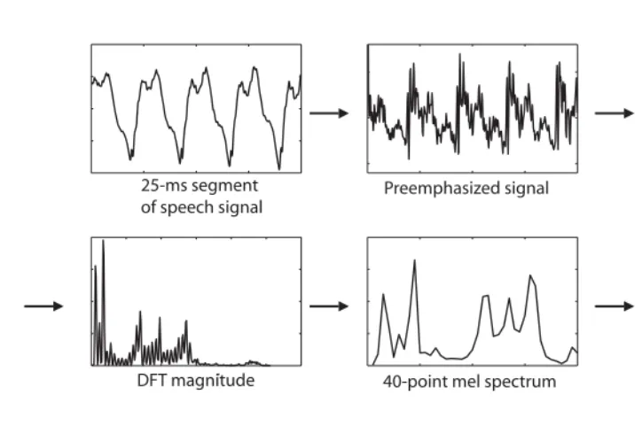
The principal mechanism for deriving feature vectors is as follows: the signal is segmented into analysis frames, typically 25-ms wide. Adjacent analysis frames are typically shifted by 10 ms with respect to one another, resulting in an analysis rate of 100 frames/s. A feature vector is derived from each frame. Specifically, the widely used mel-frequency cepstral features are obtained as follows:
1. The signal is preemphasized using a first-order finite impulse response high-pass filter to boost its high-frequency content.
2. The preemphasized signal is windowed, typically with a Hamming window [6].
3. A power spectrum is derived from it using a discrete Fourier transform (DFT) and squaring the magnitudes of the individual frequency components of the DFT.
4. The frequency components of the power spectrum are then integrated into a small number of bands using a filter bank that mimics the frequency sensitivity of the human auditory system as specified by themelscale [12], to obtain amelspectrum.
5. The mel spectral components are then compressed by a logarithmic function to mimic the loudness perception of the human auditory system.
Windowed signal
Log-mel spectrum 40-point mel spectrum
Cepstrum DFT magnitude
Preemphasized signal 25-ms segment
of speech signal
Figure 2.8 A typical example of the sequence of operations for computing mel-frequency cepstra.
An example of the above processing is shown in Figure 2.8.
Often each cepstral vector is augmented with avelocity(ordelta) term, typically computed as the difference between adjacent cepstral vectors, and anacceleration (or double-delta, ordelta-delta) term, typically computed as the difference between the velocity features for adjacent frames. The cepstral, velocity and acceleration vectors are concatenated to obtain an extended feature vector. The termsstaticanddynamicfeatures are also used to describe the cepstral features and their derivatives, respectively.
2.4.2
The HMM for a Word Sequence
The main term in Equation (2.28) is P(X|w1, w2,· · ·). We will henceforth assume that the speech recording X is a sequence of feature vectors. The probability distribution P(X|w1, w2,· · ·)is modeled using an HMM.
The HMM for each of the word sequences considered in Equation (2.28) must ideally be learned from example (or training) instances of the word sequence. The number of word sequences to consider in Equation (2.28) is typically very large, and it is usually not possible to obtain a sufficient number of training instances of each word sequence to learn its HMM properly. Therefore, we must factor the problem.