Full Terms & Conditions of access and use can be found at
http://www.tandfonline.com/action/journalInformation?journalCode=ubes20
Download by: [Universitas Maritim Raja Ali Haji] Date: 11 January 2016, At: 22:19
Journal of Business & Economic Statistics
ISSN: 0735-0015 (Print) 1537-2707 (Online) Journal homepage: http://www.tandfonline.com/loi/ubes20
Long-Horizon Return Regressions With Historical
Volatility and Other Long-Memory Variables
Natalia Sizova
To cite this article: Natalia Sizova (2013) Long-Horizon Return Regressions With Historical Volatility and Other Long-Memory Variables, Journal of Business & Economic Statistics, 31:4, 546-559, DOI: 10.1080/07350015.2013.827985
To link to this article: http://dx.doi.org/10.1080/07350015.2013.827985
Accepted author version posted online: 08 Aug 2013.
Submit your article to this journal
Article views: 167
Long-Horizon Return Regressions
With Historical Volatility and Other
Long-Memory Variables
Natalia S
IZOVADepartment of Economics, Rice University, Houston, TX 77251 ([email protected])
The predictability of long-term asset returns increases with the time horizon as estimated in regressions of aggregated-forward returns on aggregated-backward predictive variables. This previously established evidence is consistent with the presence of common slow-moving components that are extracted upon aggregation from returns and predictive variables. Long memory is an appropriate econometric framework for modeling this phenomenon. We apply this framework to explain the results from regressions of returns on risk measures. We introduce suitable econometric methods for construction of confidence intervals and apply them to test the predictability of NYSE/AMEX returns.
KEY WORDS: Long-range dependence; Return predictability; Spurious regression.
1. INTRODUCTION
Short-term asset returns (e.g., monthly) appear to be largely unpredictable. At the same time, a number of studies have demonstrated more significant predictability in long-term re-turns (e.g., annual). This increase in predictability for the ag-gregated returns occurs naturally if the predictive variables are persistent. It has become standard practice to model persistent predictive variables as stationary autoregressive processes with the high first autocorrelations (see Stambaugh1999; Boudoukh, Richardson, and Whitelaw 2008). More formally, such pro-cesses are modeled as nearly integrated (see Phillips 1988; Valkanov2003).
In this article, we compare the implications of this accepted model of persistence in predictive variables to the implications from an alternative, long-memory, model that has received less attention in the long-run predictability literature. Note that if the predictive variables are modeled as nearly integrated, then this assumption leads to exponentially decaying autocorrelations. Therefore, this model may be inadequate in at least two cases. The first case occurs when the model is used to predict the effects of small shocks to returns that decay at a rate that is apprecia-bly slower than exponential. The second case occurs when the predictive variable is only modestly persistent but may contain several slowly moving components that become manifest only upon aggregation. These two cases, on the other hand, fit nat-urally within the framework with fractionally integrated (i.e., long-memory) predictive variables (see Baillie 1996). As we will show, fractional integration has implications for the return predictability at different forecasting horizons as well as for the properties of the sample statistics in long-horizon regressions (i.e., regressions with long-term returns).
In our measurement procedure, we focus on regressions with two-way aggregation of the regressor and regressand, as pro-posed by Bandi and Perron (2008). One of the motivations for this choice is the extraction of the long-run signals from both the returns and predictive variables. We show that the popula-tionR2in these long-horizon regressions converges to zero as the horizon increases unless the predictive variables are
frac-tionally integrated. Therefore, although an increase in return predictability occurs for highly persistent (nearly integrated) short-memory processes, extreme persistence of the variables would be required for the longest horizons. Such persistence is not observed for, for example, financial volatility, term spreads, or unemployment rates. However, the behavior of these vari-ables may be consistent with the presence of long memory. We focus on the volatility of a broad stock market index, which is a particularly relevant example because, in principle, it de-pends on the same variances of the fundamental shocks that constitute the equity premium (e.g., Merton 1973; Campbell and Cochrane1999; Bansal and Yaron2004). The return pre-dictability by other measures of risk should also be analyzed within the same long-memory framework.
We present three results in this article. First, we revisit the model with nearly integrated predictive variables and adapt it to the case with volatility as a regressor. In particular, we ex-plicitly account for the heteroscedasticity in the returns and the modest size of the observed predictability over short horizons. We show that this model cannot fully account for the empiri-cal evidence in the data, such as the magnitude of the return predictability over the longest horizons. Second, we consider the predictability in the long-memory framework. We find that the increasing patterns ofR2 as a function of the horizon are inherent in this framework. However, we find that the return predictability (when present) is underestimated in small sam-ples. We derive asymptotic distributions for both models, and the resulting confidence intervals are then applied in our em-pirical study. For the volatility, we find that the long-memory model produces wider confidence intervals compared with the model with nearly integrated regressors. We, however, confirm the predictability evidence in Bandi and Perron (2008) for the longest horizons of 9 and 10 years.
© 2013American Statistical Association Journal of Business & Economic Statistics October 2013, Vol. 31, No. 4 DOI:10.1080/07350015.2013.827985
546
The article is organized as follows. Section2documents the empirical facts against which we check the validity of our econo-metric frameworks. Section3outlines a short-memory frame-work with a nearly integrated volatility and compares the impli-cations of this model with the empirical facts. Section4outlines a new framework in which the predictive variable is assumed to follow a long-memory process. Finally, we test the predictabil-ity of NYSE/AMEX returns using our asymptotic results in Section5.
2. STYLIZED EMPIRICAL FACTS
There are two pronounced empirical facts that are hard to replicate using existing models. First, the data suggest that re-turns are highly predictable over long horizons. Second, the pre-dictability of the predictive variables themselves is quite low. For illustration, we reproduce the results of the article by Bandi and Perron (2008), which analyzes the predictability of long-term NYSE/AMEX returns using volatility, and extend the original results to include 2011 data.
The data are constructed as follows. The variable to be pre-dicted is the monthly excess return,Ret,t+1=Mt
j=1rt,j−r rf t,t+1, wherert,jis thejth continuously compounded daily return (in-cluding dividends) during thetth month for the NYSE/AMEX index. These data were provided by the Center for Research in Security Prices (CRSP)/Wharton Research Data Services (WRDS) and cover the period from January 1952 to Decem-ber 2011. The risk-free rate rt,trf+1 is from the CRSP “Fama Risk-Free Rates” data file. This dataset covers the period from January 1952 to December 2011, and is based on the prices of 1 month T-bills.Mt is the number of observations in montht. The goal is to forecast future long-term returns overH peri-ods,Rt,te+H =Hi=1Rte+i−1,t+i,using the data on past realized variance (volatility) in the market:
RVt−H,t =
Note that we use the same horizonHfor the regressor RVt−H,t and for the return Re
t,t+H. This is the diagonal of the matrix reported by Bandi and Perron (2008); note that their study also provides results for different horizons of returns and volatilities. We focus only on one subset of these results because Bandi and Perron (2008) demonstrated that predictability is generally at its highest for this diagonal.
To evaluate the predictability of returns at different horizons, we run two types of regressions:
Regression A
Rt,te+H =ar+brRVt−H,t+urt+H|t, (3)
Regression B
RVt,t+H =aσ+bσRVt−H,t +uσt+H|t, (4)
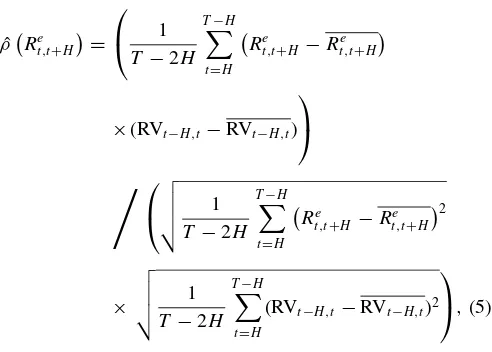
and record the corresponding correlations:
ˆ RVt−H,t over the sample that starts with observation H and ends atT −H. We use symbolfor the correlationρin (5) to indicate that this coefficient is calculated using sample data, in contrast to
ρRet,t+H=covRt,te+H,RVt−H,t
varRt,te+Hvar(RVt−H,t), which, if it exists, is a nonrandom number.
Analogously, for regression B we have
ˆ
We work with correlations to preserve the information about the sign of the relationship. The usual regression co-efficients of determination (R2) can be obtained simply as ( ˆρ(RVt,t+H))2×100% and ( ˆρ(Ret,t+H))
2
×100%. The coeffi-cients of determination for regressions A and B are reported in panel I(a) ofFigure 1, and the corresponding correlations are reported in panel II(a). Whereas ˆρ for regression A increases monotonically from approximately zero at the 1 month horizon to 0.81 at the 10 year horizon, ˆρfor regression B decreases. The percentage of the explained variation in RVt,t+H changes from 25% to nearly zero. The return predictability therefore appears to increase with the time horizon, whereas the predictability of the predictive variable itself seems to disappear.
A similar pattern is observed when we replace the real-ized volatility with another standard predictor of the long-term returns—the dividend yield, as shown in panels I(b) and II(b) of Figure 1. We continue with two-way aggregation of the regres-sor and returns, as in the volatility case. However, a difference in
0 20 40 60 80 100 120
0% 20% 40% 60%
80% 100%
Horizon (months) Panel I(a)
Return Predictability, R2 Volatility Predictability, R2
0 20 40 60 80 100 120
0% 20% 40% 60%
80% 100%
Horizon (months) Panel I(b)
Return Predictability, R2
Div.Yield Predictability, R2
0 20 40 60 80 100 120
0 0.2 0.4 0.6 0.8
1
Horizon (months) Panel II(a)
Return Predictability, ρ Volatility Predictability, ρ
0 20 40 60 80 100 120
0 0.2 0.4 0.6 0.8
1
Horizon (months) Panel II(b)
Return Predictability, ρ
Div.Yield Predictability, ρ
Figure 1. SampleR2and correlations for 1952–2011, NYSE/AMEX returns. Panel I(a) shows the sampleR2in the regressions of excess returns on past volatility and future volatility on past volatility. Panel I(b) shows the corresponding values when the dividend yield is used as the predictor. Panels II(a,b) display the corresponding sample correlations. The forecasting horizon is indicated on the OX axis.
interpretation from the previous case should be noted. While the aggregated variance overHperiods, RVt−H,t, is also a measure of theH-period variance, there is no economic motivation for the aggregation of the dividend yields. However, the aggregation can be interpreted statistically as a signal extraction procedure. This method is suitable under the assumption that the predic-tive variable contains uninformapredic-tive short-run noise, which is in effect removed through aggregation.
Figure 2 provides further details of the mechanism behind the high return predictability in long-horizon regressions by plotting future aggregated returns against the past aggregated realized variance. The figure shows how by increasing the hori-zonH, we reveal a linear relation between returns and variance at H= 10 years from the data, which, at monthly horizons, does not contain any apparent information regarding the risk relation. This exercise was performed by Bandi and Perron (2008) using a dataset that did not include the stock market crash of 2008 and led to the same findings. The fact that inclu-sion of this new data did not seem to change the concluinclu-sions
speaks to the robustness of the relation between the variance and returns.
3. ECONOMETRIC FRAMEWORK: NEARLY INTEGRATED PREDICTOR
It has been demonstrated that the analysis of long-horizon regressions such as (3) and (4) requires special methods that account for small-sample effects, which are exacerbated by the persistence of the regressors (see Ventosa-Santaul`aria 2009). To account for the persistence, Valkanov (2003) modeled pre-dictive variables as nearly integrated processes. He developed asymptotic results specifically for long-horizon regressions of asset returns.
Our first goal is to check whether this type of model can capture the long-run predictability pattern shown inFigure 1. We extend the model developed by Valkanov (2003) to volatil-ity regressors to capture various well-known facts regarding the
0 200 400 600 800 −30
−20 −10 0 10 20
H = 1 month
Excess Ret
u
rn from t to t + H
Return Variance from t − H to t
0 500 1000 1500 2000 2500
−80 −60 −40 −20 0 20 40 60
H = 12 months
Excess Ret
u
rn from t to t + H
Return Variance from t − H to t
0 500 1000 1500 2000
−100 −50 0 50 100
H = 60 months
Excess Ret
u
rn from t to t + H
Return Variance from t − H to t
500 1000 1500 2000 2500 3000
−50 0 50 100 150
H = 120 months
Excess Ret
u
rn from t to t + H
Return Variance from t − H to t
Figure 2. Effect of aggregation on return predictability. The excess returns,Re
t,t+H, are plotted versus RVt−H,Hfor the NYSE/AMEX index
from 1952 to 2011.
return–variance relationship, including leverage, heteroscedas-ticity, and positive variance:
Rt,te+1=βσt2+σtεt+1,1,
1−1+ c
T
Lb(L)(σt−μσ)=εt,2,
corr(εt,1, εt,2)=r <0. (7) The vector (εt,1, εt,2) is a martingale difference sequence. The variances ofεt,1andεt,2are normalized to one. The processvt =
b(L)−1ε
t,2satisfies a mixing condition from Herrndorf (1984):
vt is a zero-mean strong mixing sequence with mixing coeffi-cientsαm, such that∞m=1α
1−2/b
m <∞, lim supt >1E|vt|b<∞ forb >2, and the limit limT→∞E(1/T(Tt=1vt)2) exists and is positive. The initial value ofσ0is a random variable, whose distribution is independent ofT.
For this model, estimated correlations ˆρin (5) and (6) have nonstandard asymptotic distributions becauseσtbehaves similar to a unit-root process forT → ∞. To derive these distributions, we replace RVt−H,tin the definitions of the sample correlations
ˆ
ρ by its measurement-error-free analog, integrated variance, which is the sum of past variances,tt−−1Hσ
2
τ, here denoted as RVσt−H,t. The results remain the same for RVt−H,t, since under our assumptions RVt,t+H ∼Op(T2) and RVσt,t+H −RVt,t+H ∼
op(T2).
The standard assumption in the literature on overlapping observations is that H is a nontrivial portion of the sample.
Formally, it is captured by the condition limT→∞H /T =λ, 0< λ <1/2. Under this assumption, as shown in Theorem 1, ˆρ in regression A converges to a nondegenerate random variable. This result closely matches similar findings in Bandi and Perron (2008, Proposition 1).
Theorem 1. For dynamics (7), the sample correlation ˆρ in
(5) for the regression of Re
t,t+H on the past integrated vari-ancett−−1Hσ
2
τ converges weakly to the functional ˆρ(R e t,t+H)⇒
Fρ(A, B), where processesA(τ) andB(τ) are defined on the interval [λ,1−λ] as follows:
A(τ)=
τ+λ s=τ
J2,s2 ds− 1 1−2λ
1−λ λ
ζ+λ s=ζ
J2,s2 dsdζ, (8)
B(τ)=
τ s=τ−λ
J2,s2 ds− 1 1−2λ
1−λ λ
ζ s=ζ−λ
J2,s2 dsdζ, (9)
whereJ2,sis an Ornstein–Uhlenbeck (OU) process driven by a standard Brownian motionW2,s,dJ2,s=cJ2,sds+dW2,s,and
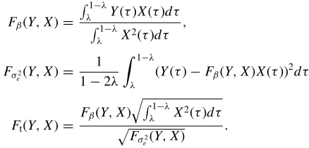
Fρis a functional of two processes that are defined and almost surely (a.s.) continuous on the interval [λ,1−λ],
Fρ(Y, X)≡
1−λ
λ Y(τ)X(τ)dτ
1−λ
λ X2(τ)dτ
1−λ
λ Y2(τ)dτ
.
The processW2,sis a limit of the partial sumsT−1/2
[T s] t=1 εt,2 when they are appropriately normalized. Therefore, the limit of
ˆ ρ(Re
t,t+H) depends only on the characteristics ofεt,2and not on
εt,1. For example, this limit remains the same if the shocks to returns are absent and excess returns are perfectly collinear with variance, which implies that ˆρ(RVσt,t+H) should converge to the same limit, that is,
ˆ
ρRVσt,t+H
⇒Fρ(A, B). (10)
The intuition behind this result is similar to that of cointegration. That is, at their limits, the long-term returnRe
t,t+Hand variance RVσt,t+Hcan be said to move in unison. Therefore, their long-run predictabilities measured by ˆρare the same. Thus, the difference in sample correlations ˆρacross these two regressions converges to zero, which clearly is not in line with the empirical obser-vations presented in Section 2. The next modification of the original model resolves this qualitative mismatch between the model and the data.
Local-to-Zero Predictability
The modification we suggest concerns the predictability of returns, namely, the parameter β. The predictability at short horizons is so small that it can be modeled as a local-to-zero predictability, that is,β =β0/T. In this section, we show that in this case, we can qualitatively match the ˆρpattern we observe in the data. That is, we can obtain high realizations of ˆρ(Rt,te+H) and a substantial difference between ˆρ(Ret,t+H) and ˆρ(RVσt,t+H). The assumption that β=β0/T allows the effect of the shock in returns to be significant, even asT → ∞. Thus, the leverage effect, which is a negative correlation between εt,1 and εt,2, influences the estimated return predictability, in accord with prior studies (Stambaugh1999). The following result is proved using the same arguments as in Theorem 1.
Theorem 2. For dynamics (7), ifβ =β0/T, the sample
cor-relation ˆρ in the regression of Re
t,t+H on the past integrated variancett−−1Hσ
rds. The asymptotic distributions of the OLS slope br and the OLS t-statistic for the slope tbr are ωT br ⇒Fβ(D, B)
The new componentC(τ) in the above theorem depends on the characteristics of the processεt,1. Therefore, under local-to-zero predictability, the limiting distribution of ˆρ(Re
t,t+h) also depends on the characteristics of the shockεt,1, in particular, on its correlation withεt,2. Correlation for the variance regression
ˆ The result of the above modifications to the original Valkanov (2003) framework is that we can now study the implications of a short-memory model that takes into account overlapping obser-vations, persistence in the predictive variable, heteroscedasticity in the returns, and the effect of a negative correlation between shocks to returns and shocks to variances. To determine if this general model can match the observed data, we consider rea-sonable values ofc, β0, ρ, andωand examine the asymptotic distribution for sample correlations.
The coefficients are chosen as follows. The persistence pa-rameter,c=(0.7−1)T, corresponds to the first autocorrela-tion of 0.7 for the monthly variances. The value of the slope is β=Re coefficient, namely, the correlation,r, is fixed at−0.76 (A¨ıt-Sahalia and Kimmel2007). For comparison, we also report the case with no leverage,r=0.
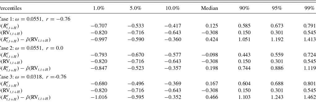
We construct the distribution of the correlation, ˆρ, in regres-sions A and B using formula (11). The results are reported in Table 1for the horizonH=120 andT =708 observations, as in Section2.Table 1shows that even asymptotically, the sample correlations can assume a wide range of values and therefore provide a poor assessment of the strengths of relationships. For example, if ω=0.0551 and r= −0.76, then the 90% prob-ability interval for ˆρ(Re
t,t+H) extends from −0.533 to 0.673. However, note that despite the high dispersion of the estimates, a value of ˆρ above 0.81 is rarely observed for regression A. Based on the data inTable 1, the probability of this event is less than 1% for all of the cases.
Another interesting observation that follows from this table is that positive and negative relations between the past volatil-ity and future returns are nearly equally likely, in contrast to the positive relation prescribed by the sign ofβ0. Indeed, the median value of ˆρ(Ret,t+H) is nearly zero in all of the cases. The distri-bution of ˆρ(Rt,te+H) is therefore centered at approximately zero, as forβ0=0, implying that 10 year horizon regressions are uninformative in testing for predictability. Note, however, that this conclusion is an outcome of the current framework with the
Table 1. Correlations ˆρ: short-memory framework with nearly integrated regressors
Percentiles 1.0% 5.0% 10.0% Median 90% 95% 99%
Case 1:ω=0.0551, r = −0.76 ˆ
ρ(Re
t,t+H) −0.707 −0.533 −0.417 0.125 0.585 0.673 0.791
ˆ
ρ(RVt,t+H) −0.820 −0.716 −0.643 −0.308 0.150 0.301 0.545
ˆ ρ(Re
t,t+H)−ρˆ(RVt,t+H) −0.997 −0.590 −0.360 0.424 1.051 1.192 1.413
Case 2:ω=0.0551, r =0.0 ˆ
ρ(Re
t,t+H) −0.793 −0.670 −0.577 −0.098 0.443 0.559 0.724
ˆ
ρ(RVt,t+H) −0.820 −0.716 −0.643 −0.308 0.150 0.301 0.545
ˆ ρ(Re
t,t+H)−ρˆ(RVt,t+H) −0.847 −0.523 −0.357 0.198 0.744 0.886 1.119
Case 3:ω=0.0318, r =-0.76 ˆ
ρ(Re
t,t+H) −0.680 −0.496 −0.369 0.167 0.604 0.688 0.801
ˆ
ρ(RVt,t+H) −0.820 −0.716 −0.643 −0.308 0.150 0.301 0.545
ˆ ρ(Re
t,t+H)−ρˆ(RVt,t+H) −1.016 −0.595 −0.352 0.466 1.103 1.243 1.462
NOTES: The table reports the percentiles for the correlations ˆρin regressions (3) and (4). The percentiles are calculated based on formulas (11) and (13), using 100,000 simulations. The integrals are calculated using 1000 steps per unit interval. It is assumed that the sample consists of 708 monthly observations, and the forecasting horizon is 120 months.
nearly integrated predictor. In the next section, we demonstrate that this finding is not accidental: for the model considered here, the unobserved true value ofρ(Rt,te +H) is in fact nearly zero for long horizons.
4. ECONOMETRIC FRAMEWORK: LONG MEMORY
How can we explain why the previous framework fails to deliver significant ˆρ(Re
t,t+H) values? One explanation is that al-though a nearly integrated process is almost nonstationary, it is still a short-memory process in small samples. This implies that although the autocorrelations of such a process are initially high, they decay at a rapid (exponential) rate. In contrast to this auto-correlation structure, long-memory processes do not necessarily exhibit high first autocorrelations, but the effect of shocks tend to persist over longer periods of time. We address this argument in this section by allowing for long-range dependence in volatility Before we turn to the details of the long-memory framework, one controversy remains to be addressed. Our assumption about the long-range dependence in variance implies a long-range dependence in the equity premium and therefore a long-range dependence in the returns. This may seem to be at odds with Rogers (1997), who showed how long memory in prices can cause a violation of the no-arbitrage condition. However, Rogers (1997, p. 104) also stated that under certain assumptions, stock prices may exhibit long-range dependence and still satisfy the no-arbitrage condition. These assumptions hold by default if the return dynamics are obtained by solving a structural asset pricing model, and naturally, asset pricing models with risk-averse investors will produce long-memory equity premium if the volatility of the dividend stream is a long-memory process. For example, Bollerslev, Sizova, and Tauchen (2012) solved for asset prices in a long-run risk model with a long-range depen-dent volatility, and the condition described by Rogers (1997) is satisfied in their model.
4.1 Long-Memory Framework: Fixed Forecasting Horizon
Fama and French (1988, p. 4) explained long-term return predictability as a process by which “the variance of expected
returns grows faster than the variance of unexpected returns.” In this section, we demonstrate the accuracy of this explana-tion when the variance exhibits long-range dependence. On the contrary, for short-memory processes, high ˆρ(Rt,te+H) for 10 year horizons cannot be explained by this accumulation of predictability.
Herein, we define a long-memory processXt(d) based on the behavior of its spectral density around zero.
Assumption 1. The spectral density of Xt(d), fx(ω), is
defined, and there exists a positive constant C such that limω→0fx(ω)|1−e−iω|2d =Cfor some 0≤d <1/2.
The above assumption definesXt(d) as a long-memory pro-cess if d >0. The same assumption defines a short-memory process whend =0. Suppose the predictive variable (i.e., real-ized variance) satisfies Assumption 1 with the parameterd≥0, that is,
RVt−1,t =Xt(d), d≥0. (14) Also suppose that the return can be represented as the sum of a predictable componentβXt(d) and the shockεt+1:
Ret,t+1=βXt(d)+εt+1, (15) where εt+1 also satisfies Assumption 1 with parameterd =0, that is, the limit of its spectral density at zero is finite. The re-sults of this section do not change if RVt−1,t is a sum ofXt(d) and noise, as long as the noise process has the integration order d′≥0 less than d. For example, this accommodates the case when RVt−1,tis just a proxy for RVσt−1,tin the model for return, and thus, the difference RVt−1,t −RVσt−1,tis the noise. Also, the results extend to the case when the returns are predicted by sev-eral variables, andXt(d) is the one with the highest integration order. Thus, the results of this section hold for the models with several risk factors, such as those seen in, for example, different versions of the long-run risk models (e.g., Bollerslev, Tauchen, and Zhou2009; Drechsler and Yaron2011).
From Lemma 2 in Appendix B, it follows that
Theorem 3. For return dynamics (14) and (15), whereXt(d) is a long-memory process satisfying Assumption 1, the population
correlationρ(Re
t,t+H) defined as
ρRt,te+H= cov
Re
t,t+H,RVt−H,H
varRe t,t+H
var(RVt−H,H)
converges to (22d
−1)×sign(β) asH→ ∞.
There is a connection between ρ(Rt,te+H) as defined above and ˆρ(Ret,t+H), defined in (5). Correlationρ(Rt,te+H) is the limit of ˆρ(Ret,t+H) asT → ∞whenHis fixed. Thus, the above ex-pression is a sequential asymptotic result.
It follows from Theorem 3 that for all short-memory models, ρ(Re
t,t+H) converges to zero. We therefore expect there to be no predictability in long-term returns and conclude that high
ˆ ρ(Re
t,t+H) can arise only due to the high dispersion of the corre-lation. In a numerical exercise with the model parameters from Table 1, we found that|ρ(Re
t,t+H)|increases up to the medium horizon of 1 year but declines to zero for longer horizons. These results can be made available upon request.
However, the logic of Fama and French’s (1988) analysis still applies to the case of long-memory processes. Due to the accumulation of predictability,|ρ(Ret,t+H)|converges to a posi-tive constant. For example, the limit ofρ(Rt,te+H) is±0.815 if d =0.43, which is a commonly found value ofdfor the realized variance in empirical work.
Long-range dependence in the predictive variables, therefore, leads to long-run predictability. Nevertheless, we are cautious in interpreting this finding because the correlation ρ is herein defined as the limit as the available data span tends to infinity, whileHis held constant. For long-horizon regressions, however,
H becomes a large portion of the total sample. We, therefore, study the behavior of the estimated ˆρunder the assumption that H /T converges toλ >0 in Section4.2.
4.2 Long-Memory Framework: Increasing Forecasting Horizon
In this section, we calculate the asymptotic distributions of correlations ˆρas normally estimated using sample covariances and variances of Ret,t+H and RVt,t+H; see (5) and (6). Simi-lar to Valkanov (2003), we assume that observations overlap; however, in contrast to Valkanov (2003), we do not make the assumption of the local-to-unity root. We instead assume that RVt,t+1exhibits long-range dependence, that is, long memory. Following the literature on long-horizon regressions, the limit-ing distributions of ˆρ(Rt,te+H) and ˆρ(RVt,t+H) are derived under the assumption thatHis large, that is, limT→∞H /T =λ >0. Suppose that we have the same model as in the previous section, that is, the dynamics of returns and variances are described by the system of Equations (14) and (15). Again, the results do not change if the realized variance is the sum of two components, Xt(d) and a less persistent noise, and if the returns are predicted by several factors, as long asXt(d) has the highest integration order among them. To derive the asymptotic result, we rely on a more restrictive definition of the stationary long-memory process based on the limiting distribution of its partial sums.
Assumption 2. For a fixedτ ∈[0,1] and 0< d <1/2,
[τ T]
i=1 (Xi(d)−μx)
T1/2+d ⇒σdW(d),τ,
whereσ2
d =limT→∞ var
(Ti=1Xi(d))
T1+2d ,μx =EXt(d), andW(d),τis a Type I fractional Brownian motion.
A fractional Brownian motion of Type I is defined in Mandelbrot and Van Ness (1968), Tsay and Chung (2000), and Marinucci and Robinson (1999) as follows:
W(d),τ =
(1+2d)Ŵ(1−d) Ŵ(1+d)Ŵ(1−2d)
τ 0
(τ −s)ddW2,s
+
0 −∞
[(τ −s)d−(−s)d]dW2,s
, (16)
wheredW2,sare increments of a standard Brownian motion. As-sumption 1 is more general than AsAs-sumption 2; for an overview of different definitions and properties of long-range dependent processes, see Baillie (1996). We now consider which models satisfy Assumption 2. Naturally, this assumption is satisfied for short-memory processes ifd =0 under the general conditions of the functional central limit theorem. For long-memory pro-cesses, a general class that satisfies Assumption 2 is that of moving-average processes.
Example 1.
Xt(d)=μx+ ∞
i=0
θiεtx−i,
where εxt are iid zero-mean shocks with a finite variance, and the sequence{θi}∞i=0decays hyperbolically (Marinucci and Robinson 2000). That is, coefficients θi decay as l(i)id−1, 0≤d <1/2 fori→ ∞, wherel(.) is a Lebesgue-measurable slow-varying function, bounded on compact subsets and posi-tive on [a,+∞) for somea >0.
Furthermore, if instead ofXt(d), only√Xt(d) can be repre-sented as a such stationary moving-average process, thenXt(d) may still satisfy Assumption 2.
Example 2.
Xt(d)=
˜ μx+
∞
i=0
θiεtx−i
2
,
where εx
t are iid Gaussian zero-mean shocks, the sequence
{θi}∞i=0satisfies the assumption from Example 1, and ˜μx=0. The fractional stochastic volatility model suggested by Comte and Renault (1998), which is one of the few available continuous-time long-memory models for financial volatility, satisfies Assumption 2.
Example 3.
Xt(d)=
t t−1
σ2(u)du,
dlnσ(t)= −κlnσ(t)dt+σ dw(d)(t),
wherew(d)(t) is a truncated fractional Brownian motion andκ > 0. This example and the previous one both satisfy the condition of nonnegativity of the variance and can be proven to satisfy Assumption 2 using the arguments of Taqqu (1975). Cases that violate Assumption 2 can also be found in Taqqu (1975).
Theorem 4. For the dynamics (14) and (15), under
Assump-and the processW(d),τ is a Type I fractional Brownian motion (16).
The above result readily follows from the continuous mapping theorem (CMT). Note that ˆρ(RVt,t+H) converges to the same limit, as the error term does not matter for the asymptotic dis-tribution of ˆρ(Rt,te+H).Table 2lists the asymptotic distribution of ˆρ(Re
t,t+H) for different levels of data aggregation,λ=H /T. For example, ifH=120 months andT =708 months, thenλ is approximately 0.17.
The data reported in Table 2 include both long-memory (d=0.43) and short-memory (d=0) cases. The second col-umn of the table lists the genuine ρ(Re
t,t+H) for large hori-zonsH, that is, its limit asH→ ∞. Ifd =0.43, then based on Theorem 3, limH→∞ρ(Ret,t+H)=0.815. For the short-memory case, the genuine long-run predictability is zero, that is, limH→∞ρ(Rt,te+H)=0. The next three columns list the median values and the 5th and 95th percentiles for the asymptotic limits of the sample ˆρ(Rt,te+H) for large horizonsHas T → ∞and H /T →λ.
A few conclusions follow fromTable 2. First, there is a nega-tive bias in ˆρ(Re
t,t+H) that increases with the aggregation param-eter,λ. Indeed, all the median values of ˆρ(Re
t,t+H) are well below the value ofρ(Re
t,t+H). In the long-memory case, for time hori-zons that constitute 1/20 of the sample (approximately 3 years in our empirical example), the median value of ˆρ(Re
t,t+H) is 0.402,
Table 2. Correlation ˆρ(Re
t,t+H): long-memory framework
ˆ
NOTES: The table reports the percentiles for ˆρin regression (3) under the assumption that limT→∞H /T=λ. The percentiles are calculated based on the long-memory framework presented in Section4.2formula (17), using 100,000 simulations. The integrals are calcu-lated using 1000 steps per unit interval. The first column shows limH→∞ρ(H)=(22d−1), which is the population equivalent of ˆρfor long horizons.
which is well below the population value of 0.815. ˆρ(Re t,t+H) decreases even further for 1/10 of the sample, corresponding to approximately a 6 year horizon, and drops below zero for 10 year horizons. The implication is that the predictability of re-turns and variances in small samples is always underestimated. Second, the accuracy of the sample correlation ˆρ(Rt,te+H) de-creases with an increase in the aggregation levelλ. For example, ifd=0.43 andHis 1/20 of the total sample, ˆρ(Rt,te+H) has a 90% probability of taking a value between−0.018 and 0.697. If
His 0.17 of the total sample, then the 90% probability interval is [−0.675,0.652].
Finally, despite the sharp decline in accuracy due to aggre-gating observations, the long-memory model results in a dis-tribution of ˆρ(Re
t,t+H) that is more often positive than negative forλ≤0.10. Simultaneously, the distribution of ˆρ(Re
t,t+H) for memory models is centered on zero. Thus, in the short-memory models, we are equally likely to observe positive and negative correlations between future returns and variances for long horizons.
Now consider the difference between the regression for re-turns (3) and the regression for volatilities (4). Up until now, the unpredictable part of the returns did not affect the result in (17) because the predictable part dominated the distribution as T → ∞. As in the short-memory local-to-unity framework, to ensure that the unpredictable part of the return affects the lim-iting distribution of ˆρ(Re
t,t+H), we introduce the local-to-zero predictability into the model as follows:
Rt,te+1= β0
TdXt(d)+εt+1. (19) Here,Xt(d) is the long-run component of the realized variance, RVt−1,t, that is, the part of the realized variance with the largest long-memory parameter, d.Xt(d) again satisfies Assumption 2 with d >0.εt+1 is a process satisfying the assumptions of the functional central limit theorem, that is, Assumption 2 with d =0, so that√1
T
[τ T]
t=1 εt+1⇒σεW1,τ, forming a multivariate fractional Brownian motion (mfBm) jointly with the limit of the partial sums of RVt−1,t. The use of mfBm as a limiting process and efficient methods for the simulation of mfBm are discussed in Amblard et al. (2011).
The new result that applies to the dynamics (19) is given by Theorem 5 and, again, can be obtained by using the CMT.
Theorem 5. For the dynamics (14) and (19), the sample fines the predictability of returns in (19), and σd is an asymptotic standard deviation for the normalized sums of Xt(d), that is, limT→∞var((
T
t=1Xt(d))/T1/2+d)=σd2, and
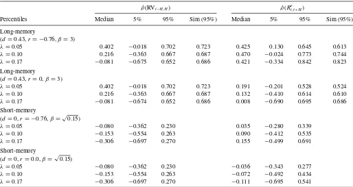
Table 3. Correlation ˆρ: long-memory framework with local-to-zero predictability
ˆ
ρ(RVt−H,H) ρˆ(Rt,te+H)
Percentiles Median 5% 95% Sim (95%) Median 5% 95% Sim (95%)
Long-memory
(d=0.43,r= −0.76,β=3)
λ=0.05 0.402 −0.018 0.702 0.723 0.425 0.130 0.645 0.613
λ=0.10 0.216 −0.363 0.667 0.687 0.470 −0.024 0.773 0.744 λ=0.17 −0.081 −0.675 0.652 0.686 0.421 −0.334 0.842 0.823
Long-memory
(d=0.43,r=0,β=3)
λ=0.05 0.402 −0.018 0.702 0.723 0.191 −0.201 0.528 0.524 λ=0.10 0.216 −0.363 0.667 0.687 0.132 −0.410 0.614 0.610 λ=0.17 −0.081 −0.674 0.652 0.686 0.008 −0.690 0.695 0.686
Short-memory
(d=0,r= −0.76,β=√0.15)
λ=0.05 −0.080 −0.362 0.230 0.035 −0.280 0.339
λ=0.10 −0.153 −0.554 0.263 0.090 −0.412 0.535
λ=0.17 −0.306 −0.697 0.270 0.155 −0.499 0.691
Short-memory
(d=0,r=0.0,β=√0.15)
λ=0.05 −0.080 −0.362 0.230 −0.036 −0.343 0.277 λ=0.10 −0.153 −0.554 0.263 −0.072 −0.492 0.434 λ=0.17 −0.306 −0.697 0.270 −0.111 −0.695 0.541
NOTES: The table reports the percentiles for ˆρin regressions (3) and (4) under the assumption that limT→∞H /T=λand for local-to-zero predictability. The percentiles are calculated based on the long-memory framework presented in Section4.2, formula (20), using 100,000 simulations. The integrals are calculated using 1000 steps per unit interval. The last column in each block, for ˆρ(RVt−H,H) and ˆρ(Rt,te+H), provides the simulated 95th percentiles in the long-memory model of Comte and Renault (1998).
σε is an asymptotic standard deviation for normalized sums of εt+1, that is, limT→∞var((Tt=1εt+1)/T1/2)=σε2. It also holds that ˆρ(RVt,t+H)⇒Fρ(Ad, Bd), the OLS slopebrTd ⇒
σε
σdFβ(Dd, Bd), and the OLSt-statistic for the slopetbr/
√
T ⇒ Ft(Dd, Bd).
Note that the leverage coefficient enters the above for-mulas only implicitly, through the correlation between the processes W1,τ and W2,τ, where the latter drives W(d),τ in (16). Letd[W1,τ, W2,τ]=rdτ. The new parameters that enter the above formulas, therefore, include the ratio (β0σd)/σε and r. The first parameter defines the variance ratio be-tween the predictable and unpredictable parts of the return process, limH→∞var(
H t=1
β0
TdXt(d))×var(
H
t=1εt+1)−1= ((β0σd)/σε)2λ2d. To select the value of (β0σd)/σε, we match the order of predictability for monthly and annual horizons. For example, if (β0σd)/σε=3 and 2d ≈1, then the return predictability is 15% for annual returns (λ=1/60) and 1.25% for monthly returns (λ=1/60/12) . These figures are similar to those reported by Drechsler and Yaron (2011) and Bollerslev, Tauchen, and Zhou (2009). For the short-memory model, the asymptotic variance ratio remains the same for all horizons. To calibrate (β0σd)/σε for the short-memory case, we match the same predictability at annual horizons so that (β0σd)/σεis fixed at√0.15.
The second parameter, namely, the correlation r, is most accurately defined as the asymptotic long-run leverage effect. Although thisr is not necessarily equal to the corresponding parameter calculated based on high-frequency observations, we use the estimate of the latter as a proxy forrand fix its value at−0.76 (A¨ıt-Sahalia and Kimmel2007). For comparison, we also report the results for the zero-leverage case (r=0).
Table 3reports the percentiles for the asymptotic distribution of ˆρ(Rt,te +H) and ˆρ(RVt,t+H) as functions of the aggregation level λ=H /T. Table 3 is formatted such that it is conve-nient to compare the short-memory and long-memory cases and the leverage (r= −0.76) and zero-leverage cases (r=0). The first three columns list the percentiles for the distribution of
ˆ
ρ(RVt,t+H). Again, we observe that for all cases, the estimated predictability in volatility is biased downward.
The next three columns report the percentiles for ˆρ(Rt,te+H). The very first observation is that the median values of ˆρ(Ret,t+H) are always larger than the median values of ˆρ(RVt,t+H). This observation agrees with the empirical findings in Section2. For example, for the long-memory case withr= −0.76, the me-dian ˆρ(RVt,t+H) and the median ˆρ(Rt,te+H) are −0.081 and 0.421, respectively, for λ=H /T =0.17. We observe this positive difference for all the cases; however, the difference
ˆ
ρ(Rt,te+H)−ρˆ(RVt,t+H) is sufficiently large only if we allow for the leverage effect. The effect of the leverage on the bias in regressions has been studied by Stambaugh (1999) for autore-gressive AR(1) predictive variables. In our framework, aggrega-tion of the data (withH >1) and long-range dependence alter the relation derived by Stambaugh (1999). However, similar results still hold. In addition to the small-sample bias of Stam-baugh (1999), the leverage also produces a large-sample effect by inducing a negative correlation between the predictable and unpredictable parts of the return.
The second observation fromTable 3is that the long-memory case can produce nonnegligible predictability in returns for long horizons. This follows from the last column of the table, which reports the 95th percentile for the distribution of ˆρ(Re
t,t+H). For example, ifλ=0.17, which approximates the level of the over-lap for the 10 year horizon, andr= −0.76, then the probability
of attaining ˆρ(Re
t,t+H)=0.81 is above 5%. This stands in con-trast to the short-memory case, for which, just as inTable 1, the same probability is less than 1%. To summarize, long mem-ory in volatility combined with the leverage effect generates high predictability in returns together with low predictability in volatility itself.
Since our conclusions are based on the magnitudes of the 95th percentiles, we next verify that the right tails of the asymptotic distributions are representative of the right tails of the small-sample distributions. The last column in each block ofTable 3 reports the 95th percentiles for correlations simulated using a model in which the regressor is a fractional long-memory pro-cess, see Comte and Renault (1998) (for simulations,T =708 months and σ2 mean affine process), with the same parameters as described above. As follows from the table, the asymptotic and the sim-ulated percentiles are within 1%–7% of each other for all the cases, and within 1%–3% forλ=0.17.
4.3 Generalization to the Multivariate Case
This section briefly discusses how the asymptotic results de-rived in Sections3and4can be generalized to the multivariate setting, in which predictive variables can be of either persistence type (nearly integrated or fractionally integrated). The assump-tions of Secassump-tions3and4can be combined into the following general condition. continuous nondegenerate vector-process with p elements in υ(τ) and one element in u(τ). Define υμ(τ)=υ(τ)−
For example,αj =2 for the square of a nearly integrated pre-dictor under the assumptions in Section3,αj =1/2+d for a fractionally integrated predictor under the assumptions in Sec-tion4, andαj =3/2 for all of the nearly integrated regressors considered by Valkanov (2003). For the last element,αp+1=1, as in Section3, if the heteroscedasticity in the returns is driven by a nearly integrated process, andαp+1=1/2, as in Section4, if the heteroscedasticity in the returns is driven by a long-memory process.
Letbr,j, 1≤j ≤p be thejth OLS slope in the regression (with intercept) ofRe
t,t+H on all of the elements in
H i=1ft−i. Let tb,j, 1≤j ≤p to be the corresponding OLS t statistic.
The proof of the next statement relies only on the subsequent application of the CMT and is, therefore, omitted.
Theorem 6. Under Assumption 3, if limT→∞H /T =λ >0,
where the subscriptsjdenote thejth element of each vector, and ϒυ,u = (j, j) denotes thejth diagonal element.
In the multivariate setting, the convergence rate for each slope, therefore, depends only on the persistence of the correspond-ing variable and the persistence of the error term. However, the persistence of the error term is understood in a somewhat non-conventional manner, as measured byαp+1 in condition (21). The slopes are consistent only for those predictors for which αj > αp+1. The opposite caseαj ≤αp+1results in the spurious regression problem. All of the OLS t statistics diverge at the same rate of√T, which depends neither onαj nor onαp+1. Be-causeαj andαp+1are scaling parameters for the partial sums of the regressor and the error term, respectively, they are, therefore, not present in standardized statistics. The limiting distribution of each individualtstatistic depends on the variance-covariance matrix of (υ(τ), u(τ))′. However, the distribution is not nor-mal and requires the simulation of multivariate processes, for example, mfBm processes for a set of long-memory variables satisfying a multivariate version of Assumption 2.
5. AN EMPIRICAL APPLICATION
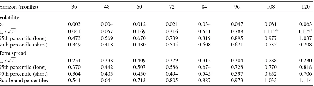
In this section, we calculate the critical values of thet statis-tics using the econometric frameworks developed in Sections3 and4.2and test for predictability in the NYSE/AMEX returns using the data and regressions described in Section 2. In test-ing the predictability of the NYSE/AMEX returns, we focus on whether long-horizon regressions yield higher power in reject-ing the null hypothesis of no-predictability.Table 4presents the OLS slopebr and the normalizedtstatistics in (3) in the first two rows. For longer horizons, all the slopes are positive, con-firming the positive risk–return relationship. The normalizedt
statistics increase as the horizon increases from 0.042 to 1.125, suggesting that the power to detect return predictability in fact increases.
The third row contains the 95th percentile for the t statis-tics based on the short-memory framework developed in Sec-tion3for the return and the realized variance withr= −0.76 (A¨ıt-Sahalia and Kimmel2007) and 1+c/T =0.7, that is, as-suming that the first autocorrelation of the monthly variances is 0.7. In contrast to the usual case of the standard normal distri-bution, the value of the 95th percentile increases with the in-crease in horizon. Thus, although the calculatedtstatistics seem higher for long-horizon regressions, their distribution under the null hypothesis also becomes more disperse. Nevertheless,
Table 4. Predictability of NYSE/AMEX returns: 1952–2011
Horizon (months) 36 48 60 72 84 96 108 120
Volatility
br 0.003 0.004 0.012 0.021 0.034 0.047 0.061 0.063
tbr/ √
T 0.041 0.057 0.169 0.316 0.541 0.788 1.112∗ 1.125∗
95th percentile (long) 0.473 0.569 0.670 0.739 0.819 0.895 0.977 1.037 95th percentile (short) 0.349 0.418 0.480 0.545 0.608 0.671 0.735 0.798
Term spread tbr/
√
T 0.234 0.338 0.409 0.379 0.313 0.304 0.288 0.280
95th percentile (long) 0.370 0.442 0.507 0.586 0.674 0.728 0.770 0.818 95th percentile (short) 0.364 0.405 0.450 0.494 0.545 0.597 0.652 0.706 Sup-bound percentiles 0.544 0.644 0.713 0.805 0.887 0.973 1.033 1.114
NOTES: The first row reportsbrin (3), where the returns are in percentage form. The second row shows the normalized OLSt-statistics in the regressions of type A (3). For the volatility,
“95th percentile (short)” indicates the asymptotic percentiles in the short-memory volatility framework described in Section3,r= −0.76 andc=(0.7−1.0)T, and “95th percentile (long)” indicates the asymptotic percentiles in the long-memory framework described in Section4,r= −0.76 andd=0.43. For the term spread, “95th percentile (short)” indicates the asymptotic percentiles in the framework of Valkanov (2003),r= −0.104 andc=(12√0.642−1.0)T(Boudoukh, Richardson, and Whitelaw2008), and “95th percentile (long)” indicates the asymptotic percentiles in the long-memory framework described in Section4,r= −0.104 andd=0.43. For the “sup-bound percentiles,” the asymptotic 95th percentiles are based on the long-memory framework withd <1/2.
comparingtstatistics with the critical values, we reject the hy-pothesis of no-predictability for returns over 8 or more years.
The fourth row of the table reports the 95th percentiles for the t statistics under the long-memory framework developed in this article. This includes the long-run correlationr= −0.76 (A¨ıt-Sahalia and Kimmel2007) and the long-memory parameter d =0.43. As follows from a comparison of the second and the third rows, the short-memory model underestimates the proba-bility of observing hightstatistics. Thus, the hypothesis of no-predictability would be overrejected if the long-memory feature of the predictive variable were not taken into account. However, based on these more conservative confidence intervals, we still conclude that the NYSE/AMEX returns are predictable using regressions for horizons of 9 and 10 years.
It is useful to compare the critical values for the long-memory and short-memory frameworks for a more persistent variable than volatility, which, in addition to high persistence, may possi-bly exhibit the long-range dependence. Therefore, we calculate the normalized tstatistics for the regression of future returns based on past term spreads. Term spread is defined as the differ-ence between long-term government bond yields and Treasury bill yields. The source of data is the same as in Boudoukh, Richardson, and Whitelaw (2008), but we consider this series at monthly frequencies and discard the data before 1952. The estimates of d for the term spread using the usual frequency-domain techniques are in the same long-memory range as for the volatility and above 0.4. We use the same “style” for regres-sions as in (3) by projecting futureH-period returns on past term spread aggregated overHmonths or, equivalently, average term spread over the previousHmonths. The normalizedtstatistics are reported in row 5 of Table 4. Their values are lower than those reported by Boudoukh, Richardson, and Whitelaw (2008) because we exclude the data prior to 1952. Nevertheless, if these
tstatistics were standard normally distributed, we would reject the hypothesis of no-predictability. Based on the short-memory and long-memory frameworks, however, as follows from com-parison of thesetstatistics with the critical values in the next two rows, there is no clear evidence that term spread predicts returns. Here, we user= −0.104, as suggested by Boudoukh, Richardson, and Whitelaw (2008). The short-memory frame-work is based on the original Valkanov model (2003) with
c=(12√0.642−1.0)T, where 0.642 is the first bias-corrected autocorrelation of term spread at annual frequencies as esti-mated by Boudoukh, Richardson, and Whitelaw (2008). For the long-memory framework,ris also −0.104 andd =0.43, which is within the range of estimates ofdfor the term spread. As follows from comparison of the 9th and 10th rows, just as in volatility case, the long-memory framework again yields more conservative critical values than the short-memory framework.
Finally, we address the issue of the critical values’ sensitivity to the choice of parameters in the long-memory framework. Un-der no predictability, the distributions of thetstatistics depend only ond, the integration order, andr, the “long-run” leverage coefficient. Both values are difficult (if not impossible) to esti-mate. Therefore, to circumvent the problem of the dependence of the statistics on these parameters, we report sup-bound 95th percentiles (see Cavanagh, Elliott, and Stock1995) of the nor-malizedtstatistics for 0≤d <1/2 andr ∈[−1,1] in the last row of the table. Even with these conservative estimates, we reject the hypothesis of no predictability in the returns for the largest horizons ofH =9 and 10 years.
6. CONCLUSION
In this work, we demonstrated that it is important to ac-count for long-range dependence in predictive variables when considering long-horizon regressions. For example, by analyz-ing the limit of the population correlation ρ(H), we showed that the long-run predictability for all short-memory models is zero, whereas the actual predictability for long-memory mod-els increases with an increase in the time horizon. That is, we demonstrated that limH→∞|ρ(H)| =22d−1, whered ≥0 is a long-memory parameter andHis a forecasting horizon.
We constructed an econometric framework that accounts for the long-memory feature in the predictive variables and de-rived the corresponding critical values oftstatistics. Based on these critical values, we tested for predictability in the long-term NYSE/AMEX returns, and we rejected the hypothesis of no-predictability for long horizons.
The “small-sample” results of our study are limited to the case of smooth dynamics, such as long-memory processes that satisfy
Assumption 2. For example, regime-switching models exhibit long-memory-like features but may not be well described by the presented econometric framework and thus remain an important topic for future research.
APPENDIX A: PROOF OF THEOREMS 1 AND 2
Proof of Theorems 1 and 2. As follows from model (7), the
dynamics of the vector (σt,ti=1εi,1) is described by the system sequence and satisfies all the assumptions forvtfrom Herrndorf (1984) that are listed in the main text.εt,1is a martingale dif-ference and C is a diagonal matrix with the elements c and 0. Consider the transformation (σ[sT]
ω√T, Brownian motion andJ2,sis a Gaussian process with correlated increments, known as the Ornstein–Uhlenbeck (OU) process:
dJ2,s=cJ2,sds+dW2,s.
Process W2,s is a standard Brownian motion such that
T−1/2[sTi=1]εi,2weakly converges toW2,s.
Now we can derive the asymptotic limit for the second (un-predictable) part of the multi-period returnHi=1σt+i−1εt+i,1. To this aim, we can apply the result of Kurtz and Protter (1991, Theorem 2.2, p. 1039), also proven in Hansen (1992, Theo-rem 2.1, p. 491), which is valid for two processes UT ,t and
VT ,t when their transformationsUT ,[sT]andVT ,[sT]jointly con-verge to processes Us and Vs for s∈[0,1]. There are also conditions on VT ,t that, for example, hold in the case when
VT ,t is a martingale with respect to the filtration to which
UT ,t andVT ,t are adapted, so that VT ,t−VT ,t−1 is a square-integrable martingale difference. These assumptions are suffi-cient for the sum[τ Ti=1]UT ,i(VT ,i+1−VT ,i) to weakly converge dictable part of the multi-period return converges to the integral fromJ2,s, The rest of the proof follows standard steps (see Valkanov 2003) and is obtained by repetitively applying the CMT.
APPENDIX B: PROOF OF THEOREM 3
A process Xt aggregated over H future periods, Ft(H)=
Lemma 1. If processXt satisfies Assumption 1 with the
pa-rameterd, correlation coefficientρ(H) converges to a function ofdas the horizonHtends to infinity,
lim
H→∞ρ(H)=2 2d
−1. (B.1)
Proof. The spectral density for the processFt(H) is equal to
fF(ω)= |1+e−iω+e−i2ω+ · · · +e−i(H−1)ω|2fx(ω)
= |1−e
−iH ω
|2 |1−e−iω|2 fx(ω).
The variance ofFt(H), which can be derived from the spectral density, equals
Substituting exponents with their trigonometric representations, we obtain
We must now find the limit of the above expression. We divide the interval [−π H, π H] into two subsets. One of them, namely, [−π Hδ, π Hδ], includes zero. We choose a value ofδthat lies in the interval 2(11+d) < δ <1. The integral over the subset that does not includex =0, normalized byH1+2d, then converges to zero asH → ∞,
The above follows from the condition that 2δ >1/(1+d) and the finite variance ofXt, that is,
π
dx. The integral then satisfies the con-dition that∀ε >0∃H0:∀H > H0
Using the same arguments as for the variance ofFt, it can be shown that
Taking into account that varFt =varPtand substituting the lim-its into the definition ofρ(H),we obtain the limit in (B.1).
Lemma 2 extends Lemma 1 to the following more general processes:
(B.2), the correlation coefficientρ(H) converges to the follow-ing function ofd:
lim
H→∞ρ(H)=(2 2d
−1)×sign(β). (B.3)
The proof follows from the same arguments as in Lemma 1 applied to processesXt,εtF, andεPt and the fact that correla-tions are restricted to the interval [−1,1]. Note that the relation betweenεF
t andεtPdoes not affect the result.
ACKNOWLEDGMENTS
The author thanks Eric Renault, Tim Bollerslev, Federico M. Bandi, and Benoit Perron for advice regarding this article. I am also thankful to the two anonymous referees and the associate editor for their useful comments. The article also benefited from discussions with seminar participants at the 2010 Joint Statisti-cal Meeting in Vancouver, Canada, the 2010 S´eminaires Marcel-Dagenais d’´econom´etrie et de macro´economie at the Universit´e de Montr´eal, Canada, the 2010 Computational Statistics and Data Analysis (CSDA) International Conference on Computa-tional and Financial Econometrics in London, UK, the 2011 North American Summer Meeting of the Econometric Soci-ety at the Washington University in St. Louis, and the 2011 Center for Research in Econometric Analysis of Time Series (CREATES) Long-Memory Symposium at the University of Aarhus, Denmark. All the remaining errors are solely mine.
[Received May 2012. Revised July 2013.]
REFERENCES
A¨ıt-Sahalia, Y., and Kimmel, R. (2007), “Maximum Likelihood Estimation of Stochastic Volatility Models,”Journal of Financial Economics, 83, 413– 452. [550,554,555,556]
Amblard, P. O., Coeurjolly, J. F., Lavancier, F., and Philippe, A. (2011), “Basic Properties of the Multivariate Fractional Brownian Motion,”S´eminaires et Congr`es, SMF, 28, 65–87. [553]
Baillie, R. T. (1996), “Long Memory Processes and Fractional Integration in Econometrics,”Journal of Econometrics, 73, 5–59. [546,552]
Bandi, F. M., and Perron, B. (2008), “Long-Run Risk-Return Trade-Offs,” Jour-nal of Econometrics, 143, 349–374. [546,547,548,549]
Bansal, R., and Yaron, A. (2004), “Risks for the Long Run: A Potential Reso-lution of Asset Pricing Puzzles,”Journal of Finance, 59, 1481–1509. [546] Bollerslev, T., Tauchen, G., and Zhou, H. (2009), “Expected Stock Returns and Variance Risk Premia,”Review of Financial Studies, 22, 4463–4492. [551,554]
Bollerslev, T., Sizova, N., and Tauchen, G. (2012), “Volatility in Equilibrium: Asymmetries and Dynamic Dependencies,”Review of Finance, 16, 31–81. [551]
Boudoukh, J., Richardson, M., and Whitelaw, R. (2008), “The Myth of Long-Horizon Predictability,”Review of Financial Studies, 21, 1577–1605. [546,556]
Campbell, J., and Cochrane, J. (1999), “By Force of Habit: A Consumption-Based Explanation of Aggregate Stock Market Behavior,”Journal of Polit-ical Economy, 107, 205–251. [546]
Cavanagh, C. L., Elliott, G., and Stock, J. H. (1995), “Inference in Models With Nearly Integrated Regressors,”Econometric Theory, 11, 1131–1147. [556] Comte, F., and Renault, E. (1998), “Long Memory in Continuous-Time Stocha-sic Volatility Models,”Mathematical Finance, 8, 291–323. [552,554,555] Drechsler, I., and Yaron, A. (2011), “What’s Vol Got to Do With It,”Review of
Financial Studies, 24, 1–45. [551,554]
Fama, E. F., and French, K. R. (1988), “Dividend Yields and Expected Stock Returns,”Journal of Financial Economics, 22, 3–25. [551,552]
Hansen, B. E. (1992), “Convergence to Stochastic Integrals for Dependent Heterogeneous Processes,”Econometric Theory, 8, 489–500. [557] Herrndorf, N. (1984), “A Functional Central Limit Theorem for Weakly
Depen-dent Sequences of Random Variables,”Annals of Probability, 12, 141–153. [549,557]
Kurtz, T. G., and Protter, Ph (1991), “Weak Limit Theorems for Stochastic Integrals and Stochastic Differential Equations,”Annals of Probability, 19, 1035–1070. [557]
Mandelbrot, B. B., and Van Ness, J. W. (1968), “Fractional Brownian Motions, Fractional Noises and Applications,”SIAM Review, 10, 422–437. [552] Marinucci, D., and Robinson, P. M. (1999), “Alternative Forms of Fractional
Brownian Motion,”Journal of Statistical Planning and Inference, 80, 111– 122. [552]
——— (2000), “Weak Convergence of Multivariate Fractional Pro-cesses,” Stochastic Processes and Their Applications, 86, 103–120. [552]
Merton, R. C. (1973), “An Intertemporal Capital Asset Pricing Model,” Econo-metrica, 41, 867–887. [546]
Phillips, P. C. B. (1987), “Towards a Unified Asymptotic Theory for Autore-gression,”Biometrika, 74, 535–547. [557]
——— (1988), “Regression Theory for Near-Integrated Time Series,” Econo-metrica, 56, 1021–1043. [546]
Rogers, L. C. G (1997), “Arbitrage With Fractional Brownian Motion,” Mathe-matical Finance, 7, 95–105. [551]
Stambaugh, R. F. (1999), “Predictive Regressions,”Journal of Financial Eco-nomics, 54, 375–421. [546,550,554]
Taqqu, M. S. (1975), “Weak Convergence to Fractional Brownian Motion and to the Rosenblatt Process,”Z. Wahrscheinlichkeitstheorie verw. Gebiete, 31, 287–302. [552]
Tsay, W. J., and Chung, F. (2000), “The Spurious Regression of Frac-tionally Integrated Processes,” Journal of Econometrics, 96, 155–182. [552]
Valkanov, R. (2003), “Long-Horizon Regressions: Theoretical Results and Applications,” Journal of Financial Economics, 68, 201–232. [546,548,550,552,555,556,557]
Ventosa-Santaul`aria, D. (2009), “Spurious Regression,”Journal of Probability and Statistics, 2009, 1–27. [548]