Scale-Dependent Functions, Stochastic Quantization
and Renormalization
Mikhail V. ALTAISKY †‡
† Joint Institute for Nuclear Research, Dubna, 141980 Russia
URL: http://lrb.jinr.ru/people/altaisky/MVAltaiskyE.html
‡ Space Research Institute RAS, Profsoyuznaya 84/32, Moscow, 117997 Russia
E-mail: [email protected]
Received November 25, 2005, in final form April 07, 2006; Published online April 24, 2006 Original article is available athttp://www.emis.de/journals/SIGMA/2006/Paper046/
Abstract. We consider a possibility to unify the methods of regularization, such as the renormalization group method, stochastic quantization etc., by the extension of the standard field theory of the square-integrable functionsφ(b)∈L2
(Rd
) to the theory of functions that depend on coordinateb and resolution a. In the simplest case such field theory turns out to be a theory of fields φa(b,·) defined on the affine groupG :x′ =ax+b, a >0, x, b ∈
Rd
, which consists of dilations and translation of Euclidean space. The fields φa(b,·) are
constructed using the continuous wavelet transform. The parameters of the theory can explicitly depend on the resolution a. The proper choice of the scale dependence g =g(a) makes such theory free of divergences by construction.
Key words: wavelets; quantum field theory; stochastic quantization; renormalization
2000 Mathematics Subject Classification: 37E20; 42C40; 81T16; 81T17
1
Introduction
In many problems of field theoretic description of infinite-dimensional systems the continuous description of fields and propagators faces the problem of infinities in loop integrals. The underlying physics is that field theoretic description includes integration over all microscopic scales smaller than the size of the system. In the simplest case small-scale fluctuations can be just averaged to get the classical equations for macroscopic fields. The best known example is the laminar flow hydrodynamics. In more complicated cases interaction strength (and even type) may depend on the scale. The examples are: turbulent fluid flow, critical phenomena, elementary particles interaction, etc.
For this reason we need a measure of integration that works better than Euclidean integration does. For some cases such measures are observed experimentally: these are fractal measure of energy dissipation in turbulent field [1,2], fractal mass distribution of percolation clusters, etc. For high energies, when the fractal distribution of the field or order parameter can not be measured experimentally due to the uncertainty principle, the search for a better measure of integration remains a mathematical problem. Fortunately, all these phenomena share a common important feature – the self-similarity, or scaling. The percolation processes in nanoelectronics, the turbulent velocity field, and the nucleon scattering – all display the same picture if being observed at different scales. The self-similarity has initiated at least two important regularization methods for field theory models:
φ(x)∈L2(Rd) by the scale-truncated fields
φ(2π Λ)(x) =
Z
|k|≤Λ
e−ıkxφ˜(k) d
dk
(2π)d, (1)
makes the coupling constants dependent on the cut-off momentum Λ, and requires that the final physical results should be independent of the introduced scale
Λ∂Λ(Physical quantities) = 0.
• Use of random processes that are self-similar by construction for the regularization of quantum field theory (QFT) models. This is known asstochastic quantization.
In present paper we summarize the both methods by introducing the fieldsφa(b) that
expli-citly depend on both position b and the scale (resolution) a. If φ(x) is considered as the wave function of a quantum particle, then the normalization R |φa(b)|2dµ(a, b) = 1, where dµ(a, b)
is the appropriate Haar measure on affine group, expresses the fact that the probability of locating the particle anywhere in space −∞ < b < ∞ changing the resolution 0 < a < ∞ is exactly one. Thus, the RG symmetry related to the change of the scaleaextends the symmetry of the theory by allowing the change of parameters with scale. Technically, construction of the scale-dependent fields φa(b) is performed by using continuous wavelet transform (CWT).
It should be noted that since field theoretic calculations are usually performed with the help of the Fourier transform the cut-off momentum Λ corresponds to the minimal coordinate scale
L= 2Λπ. However, the Fourier transform is not localized in coordinate space. For this reason we denote the fields obtained from φ(x) by truncation of the Fourier harmonics with |k|> 2Lπ (1) as φ(L)(x); in contrast to it the localized view of a function φ at the position x and the scale
a is denoted as φa(x). The mathematical meaning of the latter will be explained hereafter in
terms of wavelet transform. The same thing concerns the parameters of field theory models – masses, coupling constants, etc. In the standard approach they are dependent on the cut-off momentum and it is tacitly understood that the experimental dependence of these parameters on the squared transferred momentum Q2 is equivalent to the dependence on the cut-off. In our wavelet-based approach theg=g(a) may be the coupling constant of the given field φa(b)
of the given scale a, rather than the effective coupling constant for the harmonics of all scales up to a. For this reason different notations are used hereafter in the Fourier and the wavelet representations of field theories.
2
Wavelets and scale-dependent functions
2.1 What is wavelet transform
Wavelet transform entered mathematical physics from geophysical applications [3,4] as a prefe-rable alternative to the Fourier transform in the case when localization in both position and mo-mentum is simultaneously required. Formally the Fourier transform and the wavelet transform are on the same footing: both are decomposition of a function with respect to the representa-tions of a Lie group. However, the former uses Abelian group of translarepresenta-tions, the latter uses non-Abelian group of affine transformations
x′=aR(θ)x+b, R(θ)∈SOd, x, x′, b∈Rd.
Let us remind the general formalism. For a locally compact Lie groupGacting transitively on the Hilbert space Hit is possible to decompose vectorsφ∈ Hwith respect to the square-integrable representations U(g) of the groupG [5,6]:
|φi=Cψ−1
Z
g∈G|
where dµ(g) is the left-invariant Haar measure on G. The normalization constant Cψ is
deter-mined by the norm of the action of U(g) on the fiducial vector ψ ∈ H, i.e. any ψ∈ H that satisfies the admissibility condition
Cψ =kψk−2
Z
g∈G|h
ψ|U(g)ψi|2dµ(g)<∞,
can be used as a basis of wavelet decomposition (2).
Hereafter we assume the basic waveletψis invariant underSOdrotationsψ(x) =ψ(|x|) and
drop the angular part of the measure for simplicity (R(θ)≡1). After this simplifying assump-tion, the left-invariant Haar measure on affine group is dµ(a,b) = daddb
ad+1. The representation U(g) induced by a basic waveletψ(x) is
g:x′ =ax+b, U(g)ψ(x) =a−d/2ψ
x
−b a
. (3)
Therefore, in the Hilbert space of square-integrable functions L2(Rd), with the scalar product (f, g) :=R f¯(x)g(x)dx, a function φ∈L2(Rd) can be decomposed with respect to the represen-tations of affine group (3):
φ(x) =Cψ−1
Z
a−d/2ψ
x−b a
φa(b)dad db
ad+1 . (4)
The coefficients of this decomposition are
φa(b) =
Z
a−d/2ψ¯
x−b a
φ(x)ddx. (5)
The d-dimensional bold vector notations are dropped hereafter where it does not lead to a con-fusion, and the basic waveletψ(x) is assumed to be isotropic. Here we use normalization for the rotationally invariant wavelets
Cψ =
Z
|ψ˜(k)|2
Sd|k|d ddk,
where the area of the unit sphere in ddimensions Sdhas come from rotation symmetry.
2.2 Scale-dependent functions
Up to this point we considered only a projection of a φ∈L2(Rd) functions onto the basis con-structed of shifts and dilations of the basic wavelet ψ(x). If we substitute the inverse wavelet transform (4) into any physical theory we have started with we will reproduce it identically. However, the wavelet coefficients φa(b) may have their own physical meaning. The
convolu-tion (5) can be considered as a “microscope” that scrutinizes a field or a signalφ(x) at a pointb
at different resolutions. In this sense the functionψ can be considered as an apparatus function of the measuring device.
The most known case of such theory is the measurement of the turbulent velocity field: the mean velocity and the PDF of fluctuations of different scales should not be the same [1, 7]. Experimentally averaging of the field in a physical volumeLd is usually described as
vL=L−d
Z
Ld
K(x−y)v(y)ddy,
That is why the wavelet coefficientsφa(b) may have their own operational meaning, even if
the “no-scale” function φ(x) does not exist. In this case a sum of all fluctuations with scales equal or greater than a given scale Lcan be defined [8]:
φ(L)(x) = 2
Cψ
Z ∞
L
a−d/2ψ
x−b a
φa(b) daddb
ad+1 .
This is a close analogy to the Wilson’s RG approach to critical phenomena [9, 10, 11], where a magnetization (or velocity, or other order parameter) of scaleL is taken in the form (1).
2.3 Wavelets and random processes
If a function to be analyzed by continuous wavelet is a random function, its wavelet transform is also a random function. So, instead of the usual space of the random functions f(x,·) ∈ (Ω,A, P), wheref(x, ω)∈L2(Rd) for each given realization ωof the random process, we can go to the multiscale representation provided by the continuous wavelet transform (5):
Wψ(a,b,·) =
Z
|a|−d2ψ
x
−b a
f(x,·)ddx.
The inverse wavelet transform
f(x,·) =C−1 ψ
Z
|a|−d2ψ
x
−b a
Wψ(a,b,·) dadb ad+1
reconstructs the common random process as a sum of its scale components, i.e. projections onto different resolution spaces.
The use of the scale components instead of the original stochastic process provides extra analytical flexibility of the method: there exist more than one set of random functionsW(a,b,·)
the images of which have coinciding correlation functions in the space of f(x,·). It is easy to check that the random process generated by wavelet coefficients having in (a, k) space the correlation function
hfW(a1, k1)fW(a2, k2)i=Cψ(2π)dδd(k1+k2)a1d+1δ(a1−a2)D0
has the same correlation function as white noise has:
hf(x1)f(x2)i=D0δd(x1−x2),
hf˜(k1) ˜f(k2)i= (2π)dD0δd(k1+k2),
hfWψ(a1, k1)Wfψ(a2, k2)i= (2π)dD0δd(k1+k2)(a1a2)d/2ψ˜(a1k1) ˜ψ(a2k2).
Therefore, the space of scale-dependent random functions is just richer than the ordinary space of random functions: since we have an extra scale argumenta here, we can play with the PDF and correlations of random functions φa(b,·) to achieve required properties in ordinary space,
holding at the same time some other limitations, say, on singular behavior.
3
Stochastic quantization
3.1 Parisi–Wu stochastic quantization
Usually it is done in the functional integral formalism: if the action of the fieldφ S[φ] is known, the v.e.v. can be derived by taking functional derivatives of the generating functional
W[J(x)] =
Z
DφeıS[φ]+ıRJ(x)φ(x)dx (6)
with respect to the formal source J(x). Unfortunately, infinite perturbation series obtained by such differentiation often give infinite results and require regularization.
However, there are alternatives to this method. Since any quantum system interacts with environment, it can not be in a pure state, and averaging over all field configurations should be performed taking into account averaging over the states of environment. This can be done by considering the system environment as a thermostat, described by a Gaussian random noise; the desired v.e.v. state will be a result of relaxation to the thermodynamic limit. Thus, instead of the Feynman path integral (6), one can operate with stochastic differential equations. Because of equivalence between Euclidean QFT and the stochastic problems, the stochastic methods have found wide applications in both numeric and analytic solution of QFT problems, especially in regularization. Among those, the method of stochastic quantization of gauge fields, proposed by G. Parisi and Y. Wu [12], have been attracting attention for more than 20 years. The idea of the method is as follows. LetSE[φ] be the action Euclidean field theory inRd. Instead of direct
calculation of the Green functions from the generation functional of the field theory, it is possible to introduce a fictitious timeτ, make the quantum fields into stochastic fields φ(x) →φ(x, τ),
x ∈Rd, τ ∈ R and evaluate the momentshφ(x1, τ1). . . φ(xm, τm)i by averaging over a random
processφ(x, τ,·) governed by the Langevin equation
∂φ(x, τ)
∂τ +
δS
δφ(x, τ) =η(x, τ). (7)
The Gaussian random force is δ-correlated in both the Rdcoordinate and the fictitious time τ:
hη(x, τ)η(x′, τ′)i= 2D0δ(x−x′)δ(τ−τ′), hη(x, τ)i= 0. (8)
The physical Green functions are obtained by taking the steady state limit:
G(x1, . . . , xm) = lim
τ→∞hφ(x1, τ). . . φ(xm, τ)i.
The stochastic quantization method is much preferable to ordinary methods for it does not have problems with gauge fixing and does not require incorporation of higher derivatives as continuous regularization methods do.
Concerning the renormalization of stochastically quantized theory, the matter practically comes out to the renormalization of the Langevin equation (7) in (d+ 1) dimensions instead of renormalization of the original theory with the action functional S[φ] in d dimensions. The renormalization of the Langevin equation is usually done by constructing the characteristic functional
Z[J] =
exp
Z
ddxdτ J(x, τ)φ(x, τ)
solutions
,
where the statistical averaging h· · ·i is taken over all solutions of the Langevin equation (7). The summation over all solutions in functional integral formalism is achieved by expressing the functional δ-function as a functional integral over an imaginary auxiliary field ˆφ:
δ
∂φ(x, τ)
∂τ +
δS
δφ(x, τ)−η(x, τ)
∼
Z
Dφˆexp ˆφ
∂φ(x, τ)
∂τ +
δS
δφ(x, τ) −η(x, τ)
This is so-called Martin–Siggia–Rose field-doubling formalism [13]. The resulting theory has the form of a field theory with constraints in (d+ 1) dimensions. Under the change of the cut-off scale all fields, coordinates and parameters in such a theory are transformed according to their canonical dimensions.
The renormalization of such a theory has much in common with the renormalization of gauge theories: for the constraint (9) is similar to gauge fixing, and the functional determinant arising from the this term under the change of variables results in ghost fields and BRST symmetry. The details of renormalization of stochastically quantized theories can be found e.g. in [14,15].
3.2 Wavelet-based stochastic quantization
Taking into account the above mentioned flexibility of stochastic processes defined in the space of wavelet coefficients, it appears to be attractive to use wavelet-defined noise for stochastic quantization. Applying the wavelet transform (in spatial coordinates, but not in fictitious time)
φa(b,·) =
Z
a−dψ
x−b a
φ(x,·)ddx
to the fields and the random force in the Langevin equation (7), we get the possibility to change the white noise (8) into a scale-dependent random force
hη˜a1(k1, τ1)˜ηa2(k2, τ2)i=Cψ(2π)dδd(k1+k2)δ(τ1−τ2)a1δ(a1−a2)D(a1, k1). (10)
(Here and after we use CWT in L1 norm instead of L2.)
In the case when the spectral density of the random force is a constantD(a1, k1) =D0, the
inverse wavelet transform
φ(x) = 2
Cψ
Z ∞
0
da a
Z ddk
(2π)d dω
2π exp(ı(kx−ωτ)) ˜ψ(ak)φa(k, ω) (11)
drives the process (10) into the white noise (8).
In the case of arbitrary functions φa(x,·) we have more possibilities. In particular, we can
define a narrow band forcing that acts at a single scale
D(a, k) =a0δ(a−a0)D0. (12)
The contribution of the scales with the wave vectors apart from the the typical scalea−01 is suppressed by rapidly vanishing wings of the compactly supported wavelet ˜ψ(k).
Here we present two examples of the divergence free stochastic perturbation expansion: (i) the scalar field theoryφ3, (ii) the non-Abelian gauge field theory.
3.3 Scalar f ield theory
Let us turn to the stochastic quantization of the φ3-theory with the scale-dependent noise [16]. The Euclidean action of theφ3-theory is:
SE[φ(x)] =
Z
ddx
1 2(∂φ)
2+m2
2 φ
2+ λ
3!φ
3
.
The corresponding Langevin equation is written as
∂φ(x, τ)
∂τ +
−∆φ+m2φ+ λ 2!φ
2
Substituting the scale components in representation (11) into the Langevin equation (13) we get the integral equation for the stochastic fields:
(−ıω+k2+m2)φa(k, ω) =ηa(k, ω)− λ
2ψ˜(ak)
2
Cψ
2Z ddk
1
(2π)d dω1
2π da1
a1
da2
a2
,
˜
ψ(a1k1) ˜ψ(a2(k−k1))φa1(k1, ω1)φa2(k−k1, ω−ω1). (14)
Starting from the zero-th order approximationφ0 =G0η, with the bare Green functionG0(k, ω) =
1/(−ıω+k2+m2), and iterating the integral equation (14), we get the one-loop correction to the stochastic Green function:
G(k, ω) =G0(k, ω)
+λ2G20(k, ω)
Z ddq
(2π)d dΩ
2π2∆(q)|G0(q,Ω)|
2G
0(k−q, ω−Ω) +· · ·, (15)
where ∆(k) is the scale-averaged effective force correlator
∆(k)≡ 2
Cψ
Z ∞
0
da
a |ψ˜(ak)|
2D(a, k).
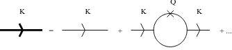
In the same way other stochastic moments are evaluated. Thus, the common stochastic diagram technique is reproduced, but with the scale-dependent random force (10) instead of the standard one (8). The diagrams corresponding to the stochastic Green function decomposition (15) are shown in Fig.1.
= + + ...
K K K K
Q
Figure 1. Diagram expansion of the stochastic Green function inφ3
-model.
It can be seen that for a single-band forcing (12) and a suitably chosen wavelet the loop divergences are suppressed. For instance, use of the Mexican hat wavelet
˜
ψ(k) = (2π)d/2(−ık)2exp(−k2/2), Cψ = (2π)d,
and the single-band random force (12) gives the effective force correlator
∆(q) = (a0q)4e−(a0q)
2
D0. (16)
The loop integrals, taken with this effective force (16), can be easily seen to be free of ultraviolet divergences at q→ ∞:
G2(k, ω) =G20(k, ω)
Z ddq
(2π)d2∆(q)
Z ∞
−∞ dΩ 2π
1
Ω2+ (q2+m2)2
1
−ı(ω−Ω) + (k−q)2+m2.
3.4 Non-Abelian gauge theory
The Euclidean action of a non-Abelian gauge field is given by
S[A] = 1 4
Z
ddxFµνa (x)Fµνa (x),
where fabs are the structure constants of the gauge group, g is the coupling constant. The Langevin equation for the stochastic quantization of gauge theory (17) can be written as
∂Aa
The two terms standing in the free field Green function correspond to the transversal and the longtitudal mode propagation:
Similarly to the scalar field theory, we can use the scale-dependent forcing (19) in the Langevin equation (18). Since there is no dynamic evolution for the longtitudal modes in the Langevin equation (18), it is natural to use the transversal scale-dependent random force
hηaa1µ(k1, τ1)ηνa2b (k2, τ2)i= (2π)dδd(k1+k2)δ(τ1−τ2)Tµν(k1)Cψa1δ(a1−a2)D(a1, k1). (19)
Let us consider a gluon loop with two cubic vertices. Summing up over the gauge group indices
ı
loop as a sum of two diagrams – those with the transversal and the longtitudal stochastic Green functions:
As it can be observed after explicit evaluation of the tensor structureslT
µν andlµνL using the force
correlator (19), and integration overdΩ, the wavelet factor in the effective force correlator ∆(q) suppresses the divergences in the case of a narrow-band forcing (12). The power factorknof the basic wavelet ψ that provides ˜ψ(0) = 0 and makes the IR behavior softer. In this respect the wavelet regularization is different from the continuous regularizationRddyRΛ(∂2)η(y, τ), which
makes UV behavior softer by the factore−k 2
Λ2, but do not affect the IR behavior, see e.g. [17].
4
Wavelet-based Euclidean f ield theory
4.1 QFT on a Lie group
Let us consider a Euclidean field theory determined by a characteristic functional
whereSE[φ(x)] is Euclidean action,N is formal normalization constant. The (connected) Green
functions (m-point cumulative moments) are evaluated as functional derivatives of the logarithm of generating functional WE[J] =e−ZE[J]:
Applying a formal partition of a unity (2) with respect to a Lie groupGwe yield a theory with the generating functional
and appropriately defined Green functions.
4.2 Wavelet-based action
Let us consider the theory of a massive scalar field with polynomial interaction
SE[φ] =
that can be alternatively interpreted as a theory of classical fluctuating field with the Wiener probability measure DP =e−SE[φ]Dφ. In this case m2 =|T−T
c|is the deviation from critical
temperature andλis the fluctuation interaction strength.
To introduce the scale-dependent fields φa(b) into the action we can just substitute the
fields φ into (20) using wavelet transform (4). For convenience and recording purposes, we rewrite continuous wavelet transform (5), (4) using theL1 norm
φa(b) =
The generating functional for the scale-dependent functions φa(b) is
W[Ja(b)] =
whereJa(b) is a formal source (“external force”), which corresponds to the fluctuations of given
scalea localized near a given pointb. The corresponding Green functions a given by
Va1...an
where integration over all pairs of matching indices daiddbi
Cψai is assumed. The inverse propagator
is the wavelet image of (−∂2+m2), that is
D(a1, a2, k) = ˜ψ(a1k)(k2+m2) ˜ψ(a2k).
As it is seen from (23), the local interaction term φn becomes nonlocal after the application of
wavelet transform (21). Of course, since the wavelet transform provides the partition of a unity, the integration over all scale arguments in the theory (22) drives it back to the original field theory with polynomial interactions, which is UV divergent. However, using the Wilson’s RG ideas we shall show how the nonlocal wavelet theory (22) can be made into a local one, which has UV finite behavior.
Let us suppose that we manage to make the wavelet theory with nonlocal interaction (23) into a local one with the coupling constant explicitly dependent on scale g=g(a). The simplest case of the fourth power interaction of this type is
Vint[φ] =
The one-loop order contribution to the Green function G2 in the theory with local
interac-tion (24) can be easily evaluated [18] by integration over a scalar variablez=ak:
Z
Therefore, there are no UV divergences forν > d−2. However, the positive values ofνmean that the interaction strengths at large scales and diminishes at small. (This is a kind of asymptotically free theory that is hardly appropriate say to magnetic systems.)
We have to admit that the idea of using wavelets for regularization and blocking of degrees of freedom has been considered by G. Battle [19] and P. Federbush [20] in lattice settings. The idea was to sum up the discrete wavelet expansion of a function starting from a large infra-red scale (set to unity) up to the infinitesimally small scale instead of integrating in Fourier space. The expansion was taken in the form
φ(x) =X
where k = (n, m, s) is a multiindex that incorporates translations and binary dilations on the lattice as well as internal degrees of freedom of the field φ, Ψk(x) forms an orthogonal basis
in L2(Rd). It have been understood then that different subgrids involved in the wavelet expan-sion (25) represent different independent degrees of freedom [21], rather than being just different approximation of the same field like that in Kadanoff block expansion. The corresponding dia-gram technique, called “wavelet diadia-grams” and originally proposed by Federbush, can be found in Battle’s book [19].
block variables hαkαk′i decrease as a high inverse power of the separation between blocks. As
a consequence of this a field theory S[φ(x)] becomes UV-finite without any renormalization. However the decoupling of interaction between different scales seems to have quite general nature and that is the reason we exploit this idea in present paper in terms of continuous
wavelet transform without using any lattices.
Now we will try to show how the local interaction of type (24) can emerge. Following K. Wilson [10,11] we consider a system of spins with spacing L0. The idea of RG applied to
a spin system is that the interaction of spins separated by a distance L0, can be substituted by
interaction of blocks (of 2d spins in each) of size 2L0 with the high-frequency details absorbed
into the interaction constants. The same procedure is then applied to the blocks of 2L0 size,
blocks of 4L0 size etc. – this is so-called Kadanoff blocking procedure. On each step of the
blocking procedure the transformation from the scaleLto 2Lis done by integrating over the high frequency degrees of freedom K > 2Lπ with appropriate adjustment of the coupling constants.
In continuous limit, i.e. in Landau theory of ferromagnetism, when spins are averaged into the mean magnetization φ(x), the energy of the spin system is given by the Ginzburg–Landau free energy functional
FE[φ] =
Z
ddx
1 2(∂φ)
2+R
2φ
2+U
4!φ
4, (26)
where integration is performed over the domain occupied by the spin system. The field theory (26) gives divergences in correlation functions. To cope with it we remind that φ(x) is the mean magnetization of a macroscopically big block, i.e. one that contains enough spins to make statistical averaging valid. This means that the fieldφshould be substituted by one containing only the fluctuations of size larger than a typical scale L:
φ(x)→φ(L)(x) =
Z
|k|<2Lπ
e−ıkxψ˜(k) d
dk
(2π)d. (27)
So, the original Ginzburg–Landau functional is made into effective action for the large-scale fields φ(L)
FL[φ(L)] = Z
ddx
1
2(∂φ(L))
2+ RL
2 φ
2 (L)+
UL
4!φ
4 (L)
, (28)
in which the effects of small-scale fluctuations with |k| ≥ 2Lπ are absorbed into the coupling constants RL and UL. It should be noted that the projection (27), performed by filtering out
the Fourier harmonics with|k| ≥ 2Lπ, is not the only possible type of smoothing: an exponential or proper-time cutoff can be used as well [22]. Similar projection can be obtained if we apply the wavelet transform with certain given kernel φ(x)→φa(b).
Wilson suggested an elegant way to determine the dependence ofRL and UL on the cutoff
scale L by averaging over fluctuations in the shell [L, L+δL) [10,9, 11]. Since we understand the fluctuations of a given scale φa(b) – now in wavelet notation – as physical fields measured
at scalea, we will reproduce the Wilson’s derivation integrating the scale-dependent free-energy
F[φa(b)] in appropriate limits over the logarithm of scale a−1da. The larger is the scale L, the
more fluctuations of smaller scales contribute to free energy.
Let L0 be the smallest size of the system – the distance between spins in the theory of
ferromagnetism. Then, the Kadanoff blocking procedure is a mapping
{ψk(0)} → {ψk(1)} → {ψk(2)} → · · ·,
where {ψ(0)k } is the basis for the finest resolution Hilbert space, with H(0)(R0, U0) being the
Hamiltonian acting on this space, {ψk(1)} is the basis of the next coarse-grained space of the resolution 2L0, etc. At each step of the coarse graining process some details are lost, so any
functionψk(1) of the basis{ψk(1)} can be expanded in the basis{ψ(0)k }; and similarly for all next
Expanding the more coarse-grained basic functions in terms of the less coarse-grained one we obtain the expansion of the parameters of the coarser Hamiltonian H(j+1) in terms of the finer HamiltonianH(j). Wilson suggested a qualitative way of doing that. Suppose we know the free
energy functional FL[φ] of scaleLand need to calculate the next coarser functionalFL+δL[φ] of
scaleL+δL. Then, we have to add fluctuations of all scales within the range [L, L+δL) to the original theory and integrate over those fluctuations. If ψ(x) is a normalized basic function of scaleL, e.g. a wave packet withk≈ 2Lπ, such that
Substituting the free energy (28) into the condition (30) and taking into account the condi-tions (29) we get
The derivation is not very rigorous, and referring the reader to the original paper [11] for the details, we just have to state that using the formal properties of Gaussian integration in (31), up to the numerical factors, we get a logarithmic contribution to the free energy
FL+δL[φ] =FL[φ] +
To derive the dependence of RL and UL on scale L two more tricks were used by Wilson:
(i) the logarithm in (32) is decomposed into a Taylor series; (ii) integration over the phase space volume corresponding to the d.o.f. related to the wavepacket ψis changed into integration over the coordinate volumeδV using the uncertainty principle.
The logarithm is decomposed into the power series only up to the second order – to get the forth order in the fields. Up to the terms that do not depend onφwe get
1
The next trick is to count the degrees of freedom corresponding to the localized wavepacketψ. Since the scales are in the range [L, L+δL), the volume in momentum space is 2δpπ ∼ δL
L2. The
phase space volume, since p≈2π/L, is
and, hence, the coordinate volume per one degree of freedom is
δV ∼ L
1+d
δL .
Thus the equation (33) can be formally multiplied by 1 =δV L−1−dδLand integrated over the
volume δV. This results in equations
RL+δL=RL+
1 2
L1−dUL−L3−dRLUL
δL,
UL+δL=UL−
3 2L
3−dU2
LδL.
See [23] for general theory of renormalization in field theory and critical phenomena.
The above Wilson’s consideration was presented only to show how integration in the thin shell below the cutoff renormalizes the parameters of the action. More rigorous formalism that accounts for the change of the action parameters by means of integration over the infinitesimally thin shell 1−δl <|q|<1 in momentum space, followed by rescaling, consists in constructing differential equations for the variation of the action functional. It is known as exact renorma-lization group (ERG). The ERG equations are rather complicated and can be found elsewhere [24, 10, 25]. If solved numerically, the ERG equations could provide exact scale dependence of the coupling constants on cutoff scale in terms of the considered model. The problems are, however, that (i) it is often impossible to solve these equations, (ii) the cutoff scale is not the same as the scale of observation, and hence it is not obvious how to interpret the ERG results; (iii) and the last, but not the least, that it is not clear how to separate the modes to be integrated over from those to be renormalized by this integration using the space of functions that depend only on momentum φ(k) ([10], Fig. 11.2). Here we propose an alternative solution of the mode separation problem: we just extend the space of functions adding the scale argument explicitly
φ(·)→φa(·).
Having the information on the dependence on scale of the effective mass RL and coupling
constantUL we can address the question, how the effective theory (28) that comprises nonlocal
interactions of all modes larger than Lcan be transformed into a theory with the local interac-tions of scales of the type (24). To do this we approximate the original Ginzburg–Landau action
F, by a new action
FE[φ] =
Z daddb
a
−12φa1(b1)Dφa2(b2) +
m2(a) 2 |φa(b)|
2+ g(a)
4! |φa(b)|
4. (34)
That meets physical requirements by construction: for a free field (g(a) = 0) it coincides with the original free action; for the interacting fields, it just satisfies the Wilson’s assumption that
only the f luctuations of the close scale interact: in the case of the action (34), certainly the equal scales only.
Since the action (34) explicitly involves integration in scale variable da/a, we can attribute the difference in the free energies (33) to interaction of the appropriate “renormalized” modes, governed by the equation (34), in the shell [L, L+δL).
Then >2 the polynomial interactions are nonlocal in wavelet space. To derive their interac-tion constant dependence on scale, we use the physical assumpinterac-tions that only the fluctuainterac-tions of close scales can directly interact to each other. So, in the self-interaction of the fieldφ
UL
Z
L
φ(x)nddx=UL
Z
L
Va1...an
b1...bn φa1(b1)· · ·φan(bn) n
Y
i=1
the terms with|lnai−lnaj| ≪1 should dominate, from where we can postulate that
It should be noted that similar idea of orthogonalization of fluctuations of different scales has been already applied to Ginzburg–Landau model by C.Best using discrete wavelet transform. However, the Best’s paper [26], having started from continuous Ginzburg–Landau model, uses
orthogonal waveletsand sufficiently strong assumptions that fluctuations of different scales are
δ-correlated in both position and scale (equation (4) from [26]). This is definitely not the case for arbitrary (non-orthogonal) wavelets and standard assumption of Gaussian nature of fluctuations in ordinary continuous model (26). Nevertheless, the Best’s idea is numerically convenient and it is interesting for what type of wavelets such behavior is really observed.
Let us perform the asymptotic estimation of the behavior of g(a) at the known behavior of UL. Let us assume that interaction takes place at the thin shell of scales [L, L+δL) and set
The important point is that in the theory (34) the observable quantities are the correlators of the scale-dependent functions hφa1(b1)φa2(b2)i. If we deal with “renormalized” action (34), where
only equal scales interact polynomially, the loop integrals can be easily evaluated for a fixed value of scale. In the fourth power interaction theory the one-loop contribution to the Green function will be
The k-dependent integral in the last equation (37) can be explicitly evaluated. As an example, let us present a “bad” case of the Morlet wavelet ˜ψ(k) = expıkz−k22, which is not admissible
For admissible wavelets (Cψ <∞) the IR behavior is milder.
5
Conclusion
In this paper we attempt to construct a theory of scale-dependent fieldsφa(b) starting from an
action functional that explicitly depends of these fields, rather than being a local functionalS[φ] truncated at certain scale L by averaging over the short-wave fluctuations |k|> 2Lπ. The diffe-rence is that in our theory it is meaningful to consider the correlation functionshφa1(b1)φa2(b2)i
between different points and different scales. This is important because any experimental mea-surement is performed not exactly in a point, but in a certain vicinity of a point, the size of which is constrained at least by the uncertainty principle: the higher momentum is used in the measurement, the smaller is the vicinity and the stronger is the perturbation caused by the measurement. Thus we have a strong need do construct a theory in terms of what is really mea-sured in experiment – scale-dependent (wavelet) fields φa(b), rather than in terms of abstract
“no-scale” functions φ(x).
Standard RG approach meets this need only partially: it enables to study the dependence of correlations on separation between points,b=b1−b2 in our terms, but not on the typical scale
of interaction. The latter is described in terms of the correlation length ξ = ξ(T), which has a universal behavior near the critical temperatureξ(T)∼(T−Tc)−ν. The Kadanoff hypothesis
that blocks of spins interact exactly as spins themselves becomes strictly valid only in critical regime ξ → ∞ at T → Tc. In other cases there are no reasons to assume that fluctuations of
different sizes do not interact to each other and hφa1(b1)φa2(b2)i = 0 for a1 6= a2, instead the
inter-scale interaction is expressed by wavelet diagrams.
As it concerns the criticality, our approach may be close to the ideas of functional self-similarity (FS) [27]: at the critical point the blocks of spins can interact with each other in the same way as primitive spins themselves, but the coupling constant is scale-covariant, i.e. its transformation with changing of scale depends on the value of coupling constant, but not on the scale.
For a quantum field theory models, which arise from the high energy physics problems, the Kadanoff block-averaging procedure can not be directly applied. Instead the universal behavior of the coupling constantg =g(a) with respect to the scale transformations a′ =eλa should be
considered as a fundamental symmetry of the physical system. Indeed, the coupling constant
g(a) is a charge of a given particle with respect to a given interaction measured at a given scalea. Since the experiments can be performed at different scalesa0 < a1< a2 <· · ·, we should expect
a universal relation between the values of charges at different scales, and it should be aninvariant charge, such thatg0≡ζ(a0, e0) =ζ(a2/a0, e2) =ζ(a1/a0, e1),or, sincee1 =ζ(a2/a1, e2),
ζ(a, g) =ζ(a/t, ζ(t, g)). (38)
The transformation of the charges between different scales (38) has a structure of the Abelian group Tt1t2 =Tt1 ◦Tt2. It describes the evolution of the coupling constant with the change of
measurement parameter – the resolution a.
In differential form the self-similarity equation (38) is most naturally expressed in the loga-rithmic coordinate l= loga:
G(l+λ, g) =G(l, G(λ, g)),
or
∂
∂l −β(g) ∂ ∂g
G(l, g) = 0, where β(g) = ∂G(λ, g)
∂λ
λ=0
.
In general case a quantity f(l, g), which is not an invariant charge, is not nullified by the generator of RG transform e−λRˆf(l, g)6=f(l, g),but the generator
ˆ
R=
∂
∂l −β(g) ∂ ∂g
determines the evolution of physical quantities under the scale transformations.
In our approach we extend the space of functionsφ(x) ∈L2(Rd) to the space of multiscale (wavelet) fieldsφa(b) for which both the positionband the scaleaare considered asindependent
variables. The RG transform therefore becomes just an Abelian subgroup of the whole symmetry group of the actionS[φa(b)] described above in this paper. The difference between our approach
and the exact renormalization group approach (ERG) consists in the fact that ERG generating functional
ZΛ[J] = Z Y
|p|≤Λ
Dφ(p)e−S[φ;Λ]−RdpJφ
is just a sum of all fluctuations truncated by a cutoff momentum Λ in their Fourier repre-sentation, and therefore having certain symmetries related to the rescaling of Λ – the cutoff
parameter. In our approach the logarithm of scalel= logabecomes an independent variable, so the technique of Lie symmetry analysis can be applied with respect tol on the same footing as with respect to the positionx. In this way the vector field that generates arbitrary transforma-tions of the action S[φa(b)] due to the transformation of dependent and independent variables
takes the form
ˆ
V =λ
∂
∂l −β(g) ∂ ∂g
+ξ ∂ ∂x +η
∂ ∂φ.
We hope that such symmetries could be used to find solutions of the wavelet renormalization equation (35).
Acknowledgement
The author is thankful to the referee for useful comments and references.
[1] Benzi R., Paladin G., Parizi G., Vulpiani A., On multifractal nature of fully developed turbulence and chaotic systems,J. Phys. A: Math. Gen., 1984, V.17, 3521–3531.
[2] Muzy J.F., Bacry E., Arneodo A., Wavelets and multifractal formalism for singular signals: application to turbulence data,Phys. Rev. Lett., 1991, V.67, 3515–3518.
[3] Zimin V.D., Hierarchic turbulence model,Izv. Atmos. Ocean. Phys., 1981, V.17, 941–946.
[4] Goupillaud P., Grossmann A., Morlet J., Cycle-octave and related transforms in seismic signal analysis,
Geoexploration, 1984/85, V.23, 85–102.
[5] Carey A.L., Square-integrable representations of non-unimodular groups, Bull. Austr. Math. Soc., 1976, V.15, 1–12.
[6] Duflo M., Moore C.C., On regular representations of nonunimodular locally compact group,J. Func. Anal., 1976, V.21, 209–243.
[7] Frish U., Turbulence, Cambridge University Press, 1995.
[8] Altaisky M.V., Scale-dependent function in statistical hydrodynamics: a functional analysis point of view,
Eur. J. Phys. B, 1999, V.8, 613–617, chao-dyn/9707011.
[9] Wilson K.G., Renormalization group and critical phenomena. II. Phase-space cell analysis of critical beha-vior,Phys. Rev. B, V.4, 1971, 3184–3205.
[10] Wilson K.G., Kogut J., Renormalization group andǫ-expansion,Phys. Rep. C, 1974, V.12, 77–200.
[12] Parisi G., Wu Y.-S., Perturbation theory without gauge fixing,Scientica Sinica, 1981, V.24, 483–496.
[13] Martin P.C., Sigia E.D., Rose H.A., Statistical dynamics of classical systems, Phys. Rev. A, 1973, V.8, 423–437.
[14] Zinn-Justin J., Renormalization and stochastic quantization,Nuclear Phys. B, 1986, V.275, 135–159.
[15] Namiki M., Stochastic quantization, Springer, 1992.
[16] Altaisky M.V., Wavelet based regularization for Euclidean field theory, in Proc. of the 24th Int. Coll. “Group Theoretical Methods in Physics” (July 2002, Paris), Editors J.-P. Gazeau, R. Kerner, J.-P. Antoine, S. Metens and J.-Y. Thibon,IOP Conference Series, 2003, V.173, 893–897, hep-th/0305167.
[17] Halpern M.B., Universal continuum regularization of quantum field theory, Progr. Theor. Phys. Suppl., 1993, V.111, 163–184.
[18] Altaisky M., φ4-field theory on a Lie group, in Proc. 4th Int. Conf. “Frontiers of Fundamental Physics”, (December 2000, Hyderabad), Editors B.G. Sidharth and M.V. Altaisky, NY, Kluwer Academic, 2001, 121–128, hep-th/0007180.
[19] Battle G., Wavelets and renormalization, World Scientific, 1989.
[20] Federbush P.G., A mass zero cluster expansion,Comm. Math. Phys., 1981, V.81, 327–340.
[21] Federbush P.G., A phase cell approach to Yang–Mills theory,Comm. Math. Phys., 1986, V.107, 319–329. [22] Gaite J., Stochastic formulation of the renormalization group: supersymmetric structure and the topology
of the space of couplings,J. Phys. A: Math. Gen., 2004, V.37, 10409–10419, hep-th/0404212. [23] Zinn-Justin J., Quantum field theory and critical phenomena, Oxford University Press, 1989.
[24] Wegner F.G., Houghton A., Renormalization group equations for critical phenomena,Phys. Rev. A, 1973, V.8, 401–412.
[25] Kubishin Yu., Exact renormalization group approach to scalar and fermionic theories, Intern. J. Modern
Phys. B, 1998, V.12, 1321–1341.
[26] Best C., Wavelet-induced renormalization group for Landau–Ginzburg model, Nucl. Phys. B Proc. Suppl., 2000, V.83–84, 848–850, hep-lat/9909151.