Some variations on Random Survival Forest
with application to Cancer Research
Arabin Kumar Dey
∗Department of Mathematics
IIT Guwahati
Assam, India - 781039
[email protected]
Anshul Juneja
Strategic Analyst
Goldman Sachs
[email protected]
September 19, 2017
Abstract
Random survival forest can be extremely time consuming for large data set. In this paper we propose few computationally efficient algorithms in prediction of survival function. We explore the behavior of the algorithms for different cancer data sets. Our construction includes right censoring data too. We have also applied the same for competing risk survival function.
1
Introducton
Random survival forest is a very popular tree-based method in predicting survival function given a set of covariates. It is a widely used algorithm in biomedical research. In this paper we introduce two new variations of Random Survival Forest and compare them with few existing variations as an application of predicting survival of a cancer patient. Extremely randomlized Tree is one popular variation of random forest. We extend similar structure in prediction of survival time. We call it as extremely randomized survival tree. We also use more ensemble structure to make much better prediction and brought more variation inside them. One popular tree based ensemble is Adaboost. It takes many weak learner additively to form a strong learner. We apply them in survival prediction. We can formulate few variations along this line. Our algorithms works in right
∗Department of Mathematics, IIT Guwahati, Assam - 781039.
censoring set up too. Modeling survival function depending on cause of the failure is an interesting dimension. This is known as competing risk models. We also extend the extra survival tree in case of competing risk.
In early eighties idea of randomized decision appeared in experimental studies. During early nineties statistical notion of variance and bias in tree models was studied by some researchers (Breiman et al. (1998), Friedman (1997)). Breiman Breiman (1996) came up in 1996 with the "Bagging" idea in order to reduce variance of a learning algorithm without increasing its bias too much. Several generic randomization methods have been proposed, like bagging, are applicable to any machine learning algorithm. In this connection, Geurts et. al. Geurts et al. (2006) introduced extremely randomized trees as a variation of Random Forest which permits to build a totally randomized random trees. Recently Adboost technique has become an attractive ensemble method in machine learning since it is low in error rate performing well in low noise data set [Thongkam et al. (2008), Ma and Ding (2003)]. The decision problem are also used in prediction
of survival function. Early experimental work by Breiman Breiman (2003) on survival forests is also relevant. In this approach a survival tree is grown using a hybrid splitting method in which nodes are split both on time and covariates. Recently Eshawaran et. al. Ishwaran et al. (2008) proposed random survival forest for analysis of right-censored survival data. But there is no work for computing survival function extending the idea of extremely randomized trees or with some ensemble techniques like Adaboost.
We organize the paper in the following way. In section 2, we provide the con-ventional structure of random survival forest. Extra survival tree and Adaboost with extra survival tree are provided in section 3. Random Survival Tree and Extra Survival Trees under Competing Risk Data is discussed in section 4. Data analysis is kept in section 5. We finally conclude in section 5.
2
Usual Structure of Random Survival forest
Like Random forest, Random survival forest builds many binary trees, but ag-gregation scheme is now based on a cumulative hazard function (CHF) described in more details below.
Steps of the random forest can be given as follows :
1. Draw bootstrap samples from the original data ntree times. For each bootstrap sample, this leaves approximately one-third of the samples out-of-bags (OOB).
2. A survival tree is grown for each bootstrap sample.
(a) At each node of the tree, select√npredictors at random for splitting. (b) Using one of the splitting criteria described below, a node is split
(c) Repeat steps (II(a) and b) until each terminal node contains no more than 0.632 times the number of events.
3. Calculate a CHF for each survival tree built. Aggregate the ntree trees to obtain the ensemble cumulative hazard estimate.
2.1
Split Criteria :
Although there are four major split criteria is available in the literature, we use log-rank based split criteria for our purpose. LR test for splitting is defined as follows :
the parent node,dti,childj is the number of events at timeti in the child nodes,
j = 1,2, Rti,childj is the number of individuals at risk at timeti in the child
nodesj= 1,2,· · · i.e. then number of individuals who are alive or dead at time
ti, andRti =Rti,child1+Rti,child2 anddti=dti,child1+dti,child2. The absolute
value ofLR(X, c)measures the node separation. The best split is chosen in such a way that it maximizes the absolute value of
LRS(X, c) =
P
xi≤cai−nµa p
n1(1−nn1)s2a
where,µa ands2a are sample mean and sample variance ofai, respectively.
LRS(X, c) measures node separation.
2.2
Ensemble CHF
Once survival reaches step-III in the algorithm, i.e. until each terminal node contain no more than 0.632 times the number of events, the trees are aggregated to form an ensemble CHF, which is calculated by grouping hazard estimates using terminal nodes. LetLbe a terminal node,ti,L be distinct survival times,
dti,L be the number of events andRti,L be the individual at risk at time (ti,L).
The CHF estimate for a terminal node L is the Nelsen-Aalen estimator.
ˆ
All individual within L will have same CHF. Forqterminal nodes in a tree, there areqdifferent CHF values. To determineLambdaˆ L(t)for an individualiwith
terminal nodeL∈Q. CHF at L would be the CHF for individual i in the test sample. The bootstrap ensemble for individual i is
Λ∗(t|xnew) =
1
ntree
ntree X
b=1
Λ∗b(t|xnew),
whereΛ∗
b(t|xnew)is CHF for a particular tree. For prediction, ensemble survival
is defined as
S(t|xnew) =e−Λ ∗(t|x
new)
3
Our Proposed Variations
We propose two variations similar to Random Survival Forest. One of the popular variation of Random Forest is extremely randomized forest or Extra Tree. The key difference between extremely randomized forest and random forest are the changes in their strategy of bringing variability in sample and covariates. Extra tree classifier takes all the sample instead of bootstrap sample, but works on randomly chosen points from the selected variables to choose the split point.
3.1
Extra Survival Trees :
We built our algorithm in predicting the survival function based on extra tree approach. We call it as Extra Survival Forest. Therefore the proposed algorithmic steps are as follows :
1. A survival tree is grown for each sample.
(a) At each node of the tree, select√npredictors at random for splitting. (b) Select set of random points to exercise splitting criteria from each
predictors.
(c) Using Log-rank splitting criteria described in previous section, a node is split using the single predictor that maximizes the survival differences between daughter nodes.
(d) Repeat steps (II(a), (b) and (c)) until each terminal node contains no more than 0.632 times the number of events.
2. Calculate a CHF for each survival tree built. Aggregate the ntree trees to obtain the ensemble cumulative hazard estimate.
3.2
Adaboost on Extra Survival Trees :
1. Input : S : training set,S=xi(i= 1,2,· · ·, n), labelsyi∈Y,k:Iterations
number.
2. for k = 1(1) K
(a) Draw random sample of size n from S with weightswi.
(b) Fit a regressorym(x)to the training data by minimizing the weighted
error function :
(d) Update the data weighting co-efficients
wmn+1=w m+1
n exp(αmI(ym(xn)6=tn))
3. Make predictions using the final model, which is given by
YM(x) = M X
m=1
αmym(x).
In the above method we choose multiple extra survival trees or multiple random survival forests to form the strong regressor YM(x). However weight
update equations are based on the weights where observations are mis-classified. Therefore the algorithm simulataneously uses classification techniques using random forest or extra trees and then finally returns the predicted value.
4
Random Survival Tree and Extra Survival Trees
under Competing Risk Data
In survival and medical studies it is quite common that more than one cause of failure may be directed to a system at the same time. It is often interesting that an investigator needs to estimate a specific risk in presence of other risk factors. In statistical literature such risk is known as competing risk model. Iswaran et al. Ishwaran et al. (2014) explored random survival forest in case of competing risk model. Competing Risks are sometimes treated little differently which depends on primary end points where it should be relapse free survival or relapse itself. To make detailed analysis we consider different data sets and carry out analysis.
1. Draw B bootstrap samples from the learning data by replacement.
2. Grow a competing risk tree for each of the bootstrap samples. Randomly select mtry predictor variables at every node of the tree. Choose the predictor variable that maximizes the competing risk splitting rule.
3. Continue tree growing as long as the number of non-censored observations in each node is larger than a pre-specified minimum terminal node size, termed node-size.
4. Calculate a cause-specific CIF and event free survival function for each tree. Average to obtain the ensemble estimates.
We propose a similar variation in the similar line using extra survival tree. The algorithm is as follows :
1. Take all training sample corresponding to a particular cause.
2. To grow a competing risk survival tree, we randomly select p candidate variables at each node of the tree.
3. Take a random split at each selected covariate to divide the data set into two groups (which will act as two daughter nodes). The node is split using the candidate variable that maximizes the cause-specific survival difference between daughter nodes.
4. Grow the tree to full size under the constraint that a terminal node should have no less thand0>0unique deaths.
5. Calculate a cause-specific CHF for each tree. Average to obtain the ensemble CHF.
4.1
Cause-specific Estimations :
In this section we discuss cause-specific cumulative incidence function (CIF), event-free survival function and cause specific cumulative hazard function. Let us assume the following :
1. t1< t2<· · ·< tmdenotem < ndistinct and ordered time to events from
(Ti)1≤i≤m
2. dj(tk) =Pni=1I(Ti=tk, δi=j)be the count of the events of typej that
have happened at time pointtk.
3. Nj(t) = Pn
i=1I(Ti ≤ tk, δi = j) be the number of type j events that
happen in time interval[0, tk].
4. d(tk) =Pjδj(tk)be the total number of failures occuring in the interval
5. N(t) =P
jNj(t)be the total number of failures occuring in the interval
[0, t].
6. Y(t) =Pni=1I(Ti≤t)be the total count of individuals which are at risk
(both event-free and uncensored) just prior to time point t.
The Nelson-Aalen estimator for the cause-specific cumulative hazard function defined byΛj(t) =EX[R
The Kaplan-Meier estimator for the event-free survival function is given by
ˆ
We use Aalen-Johansen estimator (Aalen and Johansen, 1978) to estimateFj(t)
:
We implement the algorithms in three different data sets. The codes are written using python - 2.7.6 and R - 3.3.2. All codes can be available from authors by request. The programs are run on Intel(R) Xeon(R) server with processor core 4 CPU E5620 @ 2.4GHz at Department of Mathematics IIT Guwahati.
5.1
Data Set 1 (Prediction of Survival Without
Compet-ing Risk):
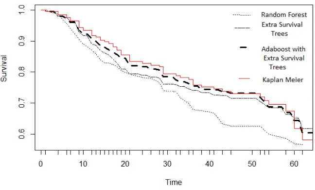
This breast cancer dataset contains gene expression and clinical data published in Desmedt et al. The data contains 198 samples to independently validate a 76 gene prognostic breast cancer signature as part of the TransBig project. In the data, 22283 gene features and 21 clinical covariates are provided for each sample. The dataset can be obtained through the R package “breastCancerTRANSBIG" of "Bioconductor".
Figure 1: Survival functions provided by different methods
5.2
Data Set 2 in Competing Risk set up : Application
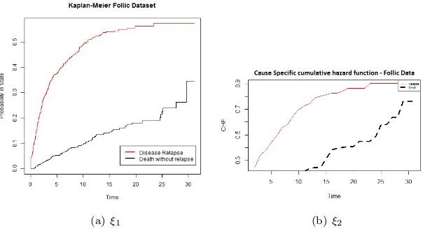
on Follicular Cell Lymphoma Data
We consider follicular cell lymphoma data from Pintilie Pintilie (2006) where additional details about data set can be found. The data set can be downloaded fromhttps://www.jstatsoft.org/article/view/v38i02, and consists of 541 patients with early disease stage follicular cell lymphoma (I or II) and treated with radiation only (chemo = 0) or a combined treatment with radiation and chemotherapy (chemo = 1). Parameters recorded were path1, ldh, clinstg, blktxcat, relsite, chrt, survtime, stat, dftime, dfcens, resp and stnum. The two competing risks are death without relapse and no treatment response. The patient’s ages (age: mean = 57 and sd = 14) and haemoglobin levels (hgb: mean = 138 and sd = 15) were also recorded. The median follow-up time was 5.5 years. There are more parameters which are not of our concern.
(a) ξ1 (b)ξ2
Figure 2: Cumulative Incidence Function based on Kaplan Meier and Extra Survival Tree
5.3
Data Set 3 : Mayo Clinic trial in Primary Biliary
Cir-rhosis (PBC) :
This dataset is available in R package survival. Originally data is collected from the Mayo Clinic trial in primary biliary cirrhosis (PBC) of the liver, conducted between 1974 and 1984. A total of 424 PBC patients, referred to Mayo Clinic during that ten-year interval, met eligibility criteria for the randomized placebo controlled trial of the drug D-penicillamine. The first 312 cases in the data set participated in the randomized trial and contain largely complete data. The additional 112 cases did not participate in the clinical trial, but consented to have basic measurements recorded and to be followed for survival. Six of those cases were lost to follow-up shortly after diagnosis, so the data here are on an additional 106 cases as well as the 312 randomized participants. Here we plot cumulative incidence function based on two competing causes ignoring the missing observation; transplant and death in Figure-3.
6
Conclusion
Predicting conditional survival function given the data set is a difficult problem. In this paper we propose extra survival tree and adaboost with extra survival tree. We implement the same for a very high dimensional data set. We develope a frame work for censoring and competing risk set up. In our algorithm we use log-rank statistic to set up split criteria. However we can use other split criteria. Our proposed algorithm take lesser time than usual random survival forest, therefore very useful for very high dimensional data set.
(a) ξ3 (b)ξ4
Figure 3: Cumulative Incidence Function based on Kaplan Meier and Extra Survival Tree
References
Breiman, L. (1996). Bagging predictors. Machine learning 24(2), 123–140.
Breiman, L. (2001). Random forests. Machine learning 45(1), 5–32.
Breiman, L. (2003). How to use survival forests. Department of Statistics, UC Berkeley.
Breiman, L. et al. (1998). Arcing classifier (with discussion and a rejoinder by the author). The annals of statistics 26(3), 801–849.
Friedman, J. H. (1997). On bias, variance, 0/1—loss, and the curse-of-dimensionality. Data mining and knowledge discovery 1(1), 55–77.
Geurts, P., D. Ernst, and L. Wehenkel (2006). Extremely randomized trees.
Machine learning 63(1), 3–42.
Ishwaran, H., T. A. Gerds, U. B. Kogalur, R. D. Moore, S. J. Gange, and B. M. Lau (2014). Random survival forests for competing risks. Biostatistics 15(4), 757–773.
Ishwaran, H. and U. Kogalur (2008). randomsurvivalforest 3.5. 1. r package.
Ishwaran, H., U. B. Kogalur, E. H. Blackstone, and M. S. Lauer (2008). Random survival forests. The annals of applied statistics, 841–860.
Ma, Y. and X. Ding (2003). Robust real-time face detection based on cost-sensitive adaboost method. InMultimedia and Expo, 2003. ICME’03. Pro-ceedings. 2003 International Conference on, Volume 2, pp. II–465. IEEE.
Molinaro, A. M., S. Dudoit, and M. J. Van der Laan (2004). Tree-based multi-variate regression and density estimation with right-censored data. Journal of Multivariate Analysis 90(1), 154–177.
Pang, H., D. Datta, and H. Zhao (2009). Pathway analysis using random forests with bivariate node-split for survival outcomes. Bioinformatics 26(2), 250–258.
Pintilie, M. (2006). Competing risks: a practical perspective, Volume 58. John Wiley & Sons.
Scheike, T. H. and M.-J. Zhang (2011). Analyzing competing risk data using the r timereg package. Journal of statistical software 38(2).
Segal, M. R. (1988). Regression trees for censored data. Biometrics, 35–47.
Thongkam, J., G. Xu, and Y. Zhang (2008). Adaboost algorithm with random forests for predicting breast cancer survivability. InNeural Networks, 2008. IJCNN 2008.(IEEE World Congress on Computational Intelligence). IEEE International Joint Conference on, pp. 3062–3069. IEEE.