Multimedia data compression Lossless compression algorithm L i l ith Lossy compression algorithm

Unit VI

M lti

di d t

i

Multimedia data compression

Lossless compression algorithm

L

i

l

ith

Introduction

„ Compression: The process of coding that will effectively

„ Compression: The process of coding that will effectively reduce the total number of bits needed to represent certain information.

„ If the compression and decompression processes induce no

A General Data Compression Scheme

„ If the compression and decompression processes induce no information loss, then the compression scheme is lossless; otherwise, it is lossy.

Basics of Information Theory

y

„ The entropy η of an information source with alphabet S = {s1,s2,...,sn} is:

Æ 2

Distribution of Gray-Level Intensities

Histograms for Two Gray-level Images Histograms for Two Gray-level Images.

Fig (a) shows the histogram of an image with uniform distribution of gray-level intensities, i.e.,

Hence, the entropy of this image is:

Entropy and Code Length

py

g

„ As can be seen in Eq (3): the entropy η is a weighted-sum of terms ; hence it represents the average amount of

i f ti t i d b l i th S

information contained per symbol in the source S.

„ The entropy η specifies the lower bound for the average number of bits to code each symbol in S, i.e.,

number of bits to code each symbol in S, i.e.,

„ -the average length (measured in bits) of the codewords produced by the encoder

(a)η=8 the minimum average (a)η=8, the minimum average

number of bits to represent each gray-level intensity is at least 8 (b)η=(1/3)log₂3 + (2/3)log₂(3/2)=0 92 (b)η (1/3)log₂3 + (2/3)log₂(3/2) 0.92

Run Length Coding

g

g

„

Memoryless Source:

an information source that is

independently distributed. Namely, the value of the

current symbol does not depend on the values of the

previously appeared symbols.

I

t

d f

i

l

R

„

Instead of assuming memoryless source,

Run-Length Coding (RLC)

exploits memory present in

the information source

the information source.

„

Rationale for RLC

: if the information source has the

property that symbols tend to form continuous

property that symbols tend to form continuous

groups, then such symbol and the length of the

group can be coded.

Variable Variable Length Coding (VLC)

g

g (

)

„ Shannon-Fano Algorithm — a top-down approach

1. Sort the symbols according to the frequency count of their occurrences.

2. Recursively divide the symbols into two parts, each with approximately the same number of counts until all parts approximately the same number of counts, until all parts contain only one symbol.

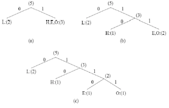
Huffman Coding

„ ALGORITHM Huffman Coding Algorithm — a bottom-up approach

1 I iti li ti P t ll b l li t t d di t th i 1. Initialization: Put all symbols on a list sorted according to their

frequency counts.

2. Repeat until the list has only one symbol left: 2. Repeat until the list has only one symbol left:

1) From the list pick two symbols with the lowest frequency counts. Form a Huffman subtree that has these two

b l hild d d t t d

symbols as child nodes and create a parent node.

2) Assign the sum of the children's frequency counts to the parent and insert it into the list such that the order is

parent and insert it into the list such that the order is maintained.

3) Delete the children from the list

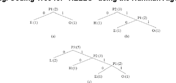
Fig. Coding Tree for "HELLO" using the Huffman Algorithm.

In Fig new symbols P1, P2, P3 are created to refer to the parent nodes in the Huffman coding tree The contents in the list are illustrated:

Properties of Huffman Coding

p

g

1. Unique Prefix Property: No Huffman code is a prefix of any other Huffman code -precludes any ambiguity in decoding.p y g y g

2. Optimality: minimum redundancy code –proved optimal for a given data model (i.e., a given, accurate, probability

distrib tion) distribution):

– The two least frequent symbols will have the same length for their Huffman codes, differing only at the last bit., g y

– Symbols that occur more frequently will have shorter Huffman codes than symbols that occur less frequently. – The average code length for an information source S is strictly less than η+ 1. Combined with Eq. (5), we have:

Extended Huffman Coding

„ Motivation: All codewords in Huffman coding have integer bit lengths. It is wasteful when pi is very large and hence

i l t 0 is close to 0.

„ Why not group several symbols together and assign a single codeword to the group as a whole?

codeword to the group as a whole?

„ It can be proven that the average # of bits for each symbol is:

Æ 7

„ An improvement over the original Huffman coding, but not much.

much.

„ Problem: If k is relatively large (e g k≥ 3) e.g., 3), then for most practical applications where n>> 1, nk implies a huge

b l t bl i ti l

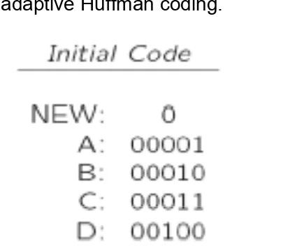
Adaptive Huffman Coding

„

Initial assigns symbols with some Initial_code

i iti ll

d

d

ith

t

i

initially agreed upon codes, without any prior

knowledge of the frequency counts.

„

_{Update tree constructs an Adaptive Human}

tree.

„

It basically does two things:

a) increments the frequency counts for the

a) increments the frequency counts for the

symbols (including any new ones).

b) updates the configuration of the tree

b) updates the configuration of the tree.

„

The encoder and decoder must use exactly

th

i iti l

d

d

d t

t

Notes on Adaptive Human Tree Updating (*)

f

f

„

Nodes are numbered in order from left to right,

bottom to top. The numbers in parentheses

i di

t

th

t

indicates the count.

„

The tree must always maintain its sibling

t

i

ll

d

(i t

l

d l

f)

property, i.e., all nodes (internal and leaf) are

arranged in the order of increasing counts.

If th

ibli

t i

b

t t b

i l t d

„

_{If the sibling property is about to be violated, a}

swap procedure is invoked to update the tree by

rearranging the nodes

Another Example: Adaptive Huffman Coding

p

p

g

„

This is to clearly illustrate more

implementation details We show exactly sent

implementation details. We show exactly sent

to simply what bits are sent, as opposed

stating how the tree is updated

stating how the tree is updated.

„

An additional rule: if any character/symbol is

t b

t th fi t ti

it

t b

d d

to be sent the first time, it must be preceded

by a special symbol NEW The initial code

b l NEW f

NEW i 0 Th

t f

„ Table 7.4 Sequence of symbols and codes sent to the decoder

„ It is important to emphasize that the code for a particular

„ It is important to emphasize that the code for a particular symbol changes during the adaptive Huffman coding

process.

„ For example, after AADCCDD, when character D overtakes A as the most frequent symbol, its code changes from 101 to 0.

Dictionary based Coding

LZW fi d l th d d t fi d t

„ LZW uses fixed-length codewords to fixed represent

variable-length strings of symbols/characters that commonly occur together, e.g., words in English text.g g g

„ the LZW encoder and decoder build up the same dictionary dynamically while receiving the data.

LZW l l d l d i i

„ LZW places longer and longer repeated entries into a

dictionary, and then emits the code for an element rather than the string element, itself, if the element has already g , , y been placed in the dictionary.

„ The predecessors of LZW are LZ77 and LZ78, due to Jacob Zi and Abraham Lempel in 1977 and 1978

Jacob Ziv and Abraham Lempel in 1977 and 1978.

„ Terry Welch improved the technique in 1984.

„ LZW is used in many applications such as UNIX compress

„ Example 2 LZW compression for string “ABABBABCABABBA”

„ • Let's start with a very simple dictionary (also referred

"table") initially containing only 3 characters with codes astable ) initially containing only 3 characters, with codes as follows:

Now the input string is ABABBABCABABBA” the LZW

Arithmetic Coding

„ Arithmetic coding is a more modern coding method that usually out-performs Huffman coding.

„ Huffman coding assigns each symbol a codeword

which has an integral bit length. Arithmetic coding can treat the whole message as one unit

treat the whole message as one unit.

„ A message is represented by a half-open interval [a, b) where a and b are real numbers between 0 and 1.

Initially, the interval is [0, 1). When the message

becomes longer the length of the interval shortens and the number of bits needed to represent the interval

Example: Encoding in Arithmetic Coding

PROCEDURE 2 Generating Codeword for Encoder

The final step in Arithmetic encoding calls for the generation of a number that falls within the range [low, high). The above algorithm will ensure that the

Lossless Image Compression

„ Approaches of Differential Coding of Images:

– Given an original image I(x, y), using a simple difference operator we can define a difference image d(x y) as

operator we can define a difference image d(x, y) as follows:

d(x, y)= I(x, y) − I(x − 1,y) Æ 9

or use the discrete version of the 2-D Laplacian operator to define a difference image d(x, y) as

d( ) 4 I( ) I( 1) I( 1) I( 1 ) I( d(x, y)=4 I(x, y) − I(x, y − 1) − I(x, y +1) − I(x +1,y) − I(x −

1,y) Æ 10

„ Due to spatial redundancy existed in normal images I, the

„ Due to spatial redundancy existed in normal images I, the difference image d will have a narrower histogram and

Lossless JPEG

„ Lossless JPEG: A special case of the JPEG image

„ Lossless JPEG: A special case of the JPEG image compression.

„ The Predictive method

1. Forming a differential prediction: A predictor combines the values of up to three neighboring pixels as the

predicted value for the current pixel indicated by 'X' in predicted value for the current pixel, indicated by 'X' in Fig. 10. The predictor can use any one of the seven schemes listed in Table 6.

2. Encoding: The encoder compares the prediction with the actual pixel value at the position `X' and encodes the difference using one of the lossless compression

difference using one of the lossless compression

Fig 10: Neighboring Pixels for Predictors in Lossless JPEG

„ Note: Any of A, B, or C has already been decoded before it is used in the predictor, on the decoder side of an

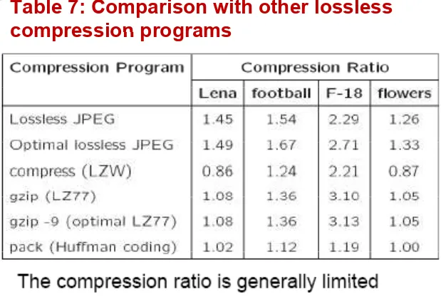
Table 7: Comparison with other lossless

compression programs

Introduction

„ Lossless compression algorithms do not deliver compression ratios that are high enough. Hence, most multimedia

compression algorithms are lossy. compression algorithms are lossy.

„ What is lossy compression ?

– The compressed data is not the same as the original data, but a close approximation of it.

– Yields a much higher compression ratio than that of lossless compression

The Rate-Distortion Theory

„

Provides a framework for the study of

Quantization

„

Reduce the number of distinct output

values to a much smaller set.

„

Main source of the “loss” in lossy

compression.

p

„

_{Three different forms of quantization.}

Uniform: midrise and midtread quantizers

– Uniform: midrise and midtread quantizers.

– Nonuniform: companded quantizer.

Uniform Scalar Quantization

„

A uniform scalar quantizer partitions the domain of

input values into equally spaced intervals, except

ibl

t th t

t

i t

l

possibly at the two outer intervals.

– The output or reconstruction value corresponding to

each interval is taken to be the midpoint of the

each interval is taken to be the midpoint of the

interval.

– The length of each interval is referred to as the

g

step

p

size, denoted by

the symbol

∆

.

„

Two types of uniform scalar quantizers:

„

Companded quantization is

nonlinear.

„

As shown above, a compander consists of

a compressor function G, a uniform

quantizer, and an expander function G

−1

.

„

_{The two commonly used companders are}

_y

_p

Vector Quantization (VQ)

„

According to Shannon’s original work on

information theory, any compression system

performs better if it operates on vectors or groups

of samples rather than individual symbols or

samples

samples.

„

Form vectors of input samples by simply

concatenating a

number of consecutive samples

concatenating a

number of consecutive samples

into a single vector.

„

Instead of single reconstruction values as in scalar

„

Instead of single reconstruction values as in scalar

Transform Coding

„

_{The rationale behind transform coding:}

If Y is the result of a linear transform T of the input

t

X i

h

th t th

t

f Y

vector X in such a way that the components of Y are

much less correlated, then Y can be coded more

efficiently than X.

efficiently than X.

„

_{If most information is accurately described by the first}

few

components of a transformed vector, then the

remaining components can be coarsely quantized, or

even set to zero, with little signal distortion.

Di

t C

i

T

f

(DCT)

ill b

t di d fi t

„

_{Discrete Cosine Transform (DCT) will be studied first.}

Spatial Frequency and DCT

„

Spatial frequency indicates how many times pixel

values

change across an image block.

„

The DCT formalizes this notion with a measure of

how much

the image contents change in

correspondence to the number of cycles of a cosine

correspondence to the number of cycles of a cosine

wave per block.

„

The role of the DCT is to decompose the original

„

The role of the DCT is to decompose the original