Chemotaxis-Inspired Load Balancing
Geoffrey Canright
1 ⋆⋆, Andreas Deutsch
2, and Tore Urnes
11
TELENOR Reseach and Development, Fornebu, Norway. geoffrey.canright,[email protected]
2
Center for High Performance Computing, Dresden University of Technology, Dresden, Germany. [email protected]
Abstract
We present an approach to the problem of load balancing on networks of nodes. Our approach is inspired by the phenomenon of negative chemotaxis in living systems. We use a diffusing signal (which is emitted by load, and moves faster than the load) to guide the movement of load towards the balanced state. Our reference system (for comparison) is unguided, diffusing load, moving at the same speed. Our tests show that the chemotaxis system can give large improvements over the reference system in convergence speed, as well as showing much reduced sensitivity to variations in network topology and in initial load distribution.
Short title: Chemotaxis-Inspired Load Balancing
Keywords: Load balancing, diffusion, chemotaxis, adaptivity, bio-inspired engineeering
1
Introduction
The problem of load balancing is quite general. Technological applications include balancing process-ing jobs among parallel processors [1]; balancprocess-ing processprocess-ing among distributed computers in a grid processing system—either peer-to-peer [2], or otherwise [3]; and balancing storage among networked storage devices [4]. There are also non-technological instances of load balancing. One of the very simplest may be taken from physics. That is, diffusion is a primitive mechanism which quite reliably seeks to distribute particles so as to move them from non-uniform states to uniform states. Fur-thermore, this is accomplished in a fully decentralized, even “unintelligent”, manner, using only the random thermal motion of the particles.
One finds load balancing also in biological systems. One example is the use of chemical repellents to prevent growth of yeast colonies into one another’s space [5]. The fact that bacteria are able to communicate with each other changed our general perception of many single, simple organisms inhabiting our world. As well as releasing the signalling molecules, yeast cells are also able to measure the number (concentration) of the molecules within a population. The term ’Quorum Sensing’ (QS) is used to describe the phenomenon whereby the accumulation of signalling molecules enable a single cell to sense the number of bacteria (cell density) and to behave accordingly.
This kind of territorial load balancing also occurs with larger organisms. In most cases, some kind of signal (urine, bird songs) is used to maintain distance between individuals or groups. Hence, in general, load balancing in biological systems is more active than the correspondingly passive, physical mechanism of diffusion. We note also that living systems are distinguished from most nonliving ones
⋆⋆Corresponding author’s address: Telenor R&D, B6d, Snarøyveien 30, 1331 Fornebu, Norway Phone: +47-91815638
Fax: +47-96211086
by being able to perform the opposite of load balancing. That is—again using active mechanisms— living systems can establish and maintain highly non-homogeneous states; examples include processes such as aggregation, morphogenesis, and self-repair.
We are interested in the problem of designing distributed, self-managing systems for solving tech-nological problems. Also, as members of the BISON [6] project, we focus on biologically-inspired solutions to such problems. In this work, we wish to explore and evaluate a mechanism for load balancing in distributed systems. This mechanism is rather directly inspired by a common biolog-ical mechanism for controlling the aggregate behavior of many small entities, namely, chemotaxis. Chemotaxis means the control of movement (taxis) via diffusive chemical signals. It is used in bi-ology both for bringing about homogeneous distributions (negative or repulsive chemotaxis), and for inducing highly non-homogeneous aggregates (positive chemotaxis) [7, 8]. In particular, chemotaxis is essential for guiding cells in biological development, the process of wound healing, and tumour an-giogenesis (a process by which a tumour is able to guide the growth of neighbouring vasculature into its own direction). Here we will implement a form of repulsive chemotaxis on a networked system, with the aim of bringing about time-efficient load balancing.
An essential aspect of chemotaxis is that the signal can diffuse faster than the bodies which are guided by the signal. In other words, there are two distinct time scales in operation in chemotaxis. This notion of two time scales is central to our thinking. Specifically, we assume that the load (which we specify only as an abstract, real-valued quantity at each node of the network) has a natural rate of movement that is significantly lower than that for the signal. We believe that, when this two-time-scale picture is correct, the use of signal can significantly speed up the movement of load towards a uniform (balanced) distribution. To put this picture into more relevant technological terms, we might suppose that the load is stored data, on the order or megabytes or gigabytes, while the signal is an indicator requiring only a few bytes. Then—possibly with the addition of prioritized queueing—we can assume that signalling data moves over the network much faster than load.
Given then that signal moves faster than load, we expect the effect of the signal to be a speedup of convergence to the balanced state. That is, we can imagine a system without signal. Repulsion or attraction can still be turned on whenever the bodies come into direct contact with one another. For example, the growing yeast colonies can stop growing when they contact others; or, in the attractive case, the amoebae of slime molds [9,10] can stick together when they come into contact. Conceivably, this mechanism can also achieve the desired distribution—but on a much longer time scale, since the movement of the amoebae is “blind” until they actually contact others. In fact, the (load balancing or aggregating) system, without signal, accomplishes redistribution via collisions; hence it works in much the same way as diffusion, with particle movement being completely “blind” between collisions. Based then on our understanding of the utility of chemotaxis in living systems, we will use “blind” movement of load as our reference system. That is, we will compare a signal-aided load balancing system on a network with a passive load balancing process, which simply uses the network equivalent of plain diffusion. Our aim in making this comparison is simple: we wish to test the hypothesis that the mechanism of chemotaxis (with its two time scales) can significantly enhance the speed of convergence of load to the uniform state, with respect to the same system operating without signalling. And we are saying here that the “same” system, without signals, is plain diffusion.
We will make this comparison more precise below. The principal idea is to ensure that the load has the same time scale, or in other words the same speed of movement, both when it is influenced by signal, and when it is not. We call this our “fairness criterion”. Given a precise prescription for ensuring this kind of fairness, we can then test whether chemotactic signalling does in fact enhance the approach to convergence for load balancing.
The use of diffusion methods for load balancing on networks has however a considerable history. One of the earliest works is that of Cybenko [11], who gave constraints for keeping the load strictly positive, and then derived some stability criteria. Cybenko also looked at linear modifications of the adjacency matrix as a way of speeding up convergence. There has been considerable subsequent work on diffusion-like mechanisms for load balancing [12–18]. A recent survey of diffusive load balancing may be found in [19]. It is in fact the simplicity and decentralized nature of diffusion that makes it attractive for handling large and/or dynamic networks, where optimization based on global information is not practical. Our aim here is to see if chemotaxis can retain the good features of diffusion, while offering significant imporvement in performance and flexibility.
The remainder of this paper is organized as follows. In section 2 we develop equations for our two algorithms—plain diffusion and chemotaxis. Also, we derive a fairness criterion in this section. Then, in section 3, we specify a number of details which are needed to translate our general equa-tions into specific implementaequa-tions for discrete-time, networked systems. Section 3 gives our basic algorithm for plain, slow diffusion, and then goes on to give a detailed discussion of our studies of
fast diffusion. This problem merits some attention, since we wish to find a stable method for fast
diffusion of signal; and it is known, at least since the work of Cybenko [11], that such a problem is nontrivial for discrete-time systems on a discrete space (network). Finally, in this section, we give the details for the two-component, coupled system that represents chemotactic load balancing. Next, in Section 4, we evaluate the performance of chemotactic load balancing with respect to our reference system (unguided diffusion of slow-moving load). Here we find some encouraging confirmation of our hypothesis—that “smart” (signal-aided) diffusion can give faster, or even much faster, convergence than “dumb” diffusion. Section 5 then addresses the question of the adaptivity of the chemotactic system. That is: being both decentralized and “smart”, such a system might be expected to also be adaptive—to variations in network topology, initial load distribution, etc. In section 5 we will offer some limited answers to this question. We also include a section (section 6) on the remarkably com-plex behavior over time that we have observed for this simple, two-component (chemotactic) system. Its behavior stands in marked contrast to the smooth, predictable behavior of slow, single-component diffusion for the same network topology. Finally, in section 7 we offer a summary.
2
Chemotaxis
First we define our terminology. We letφi represent the load at nodei. We will normally enforce
the constraint thatφi ≥0for alliand for all times. We will also assign to each node a capacityCi.
Then the load balancing problem is to seek to minimize the difference between load and capacity at each node. For this exploratory study, we set all capacities to one, and choose start distributions so that total load equals total capacity for the network. Thus the converged state is a uniform distribution with allφi = 1.
Now we address plain diffusion. The physical mechanism of diffusion, when mapped onto a discrete (space and time) system, may be expressed quite simply: nodes simply send out a fraction of what they have, at each time step, in all “directions” (to each neighbor). The fraction is then the “diffusion constant” c; while what the nodes have to send is quantified as φi −Ci. Hence, for the
simplest version of plain diffusion, a nodeiwith loadφiand capacityCiwill send a small fractionc
of its excess load(φi−Ci)to each of its neighbors, independent of node, of neighbor, and of time.
Each transfer of load to a neighbor nodejcan then be captured by the following equation:
This is our basic equation for discrete diffusion. In the next section, we will address a number of modifications to this “most simple” form of diffusion, so as to keep the load at each node positive, to enforce that transferred load is also positive, and also to allow for very fast diffusion without instabilities.
Now we introduce signal. For the signal to be useful, it must (i) move faster than load, and (ii) give information to distant nodes about the load distribution. Hence we want the load itself to “emit” signal, which then diffuses away, bringing useful information to distant nodes. Let us defineSi to be
the signal level at nodei. Then our emission equation is
∆Siemit=c2·(φi−Ci) . (2)
This emission event occurs at every time step. In fact, each equation in this section is to be imple-mented once in each time step.
It is clear from Eq. (2) that, unless total load equals total capacity, the total signal will grow (in absolute value) steadily over time. Such growth may be useful in dynamic situations where the local signal level (not the gradient) gives information which may guide a decentralized mechnism for deciding how much new load may be accepted. However in this study we focus on the static case; and to avoid divergence of the average signal level, we set total load equal to toal capacity.
Now we want the load to be guided by the signal. Specifically, we let the load respond to local signal gradients, as follows:
∆φi→j =c3·(Si−Sj) . (3)
This equation makes the movement of load less blind, and hence (we believe) more smart, than that due to plain diffusion.
Finally, we need to arrange for fast diffusion of signal. The fast versions that we develop for plain diffusion will be used to guide the movement of signal in the two-component case. Hence, the signal diffusion equation may be written analogously to Eq. 1, as follows:
∆Si→j =c4·Si . (4)
Note that no reference to capacity is needed here–signal in fact diffuses blindly.
Equation (1) thus defines our rule for the one-component case—plain diffusion of load. Equations (2—4) give the rules for the two-component case. We require some more work however before we can implement these rules. For one thing, we have, from these four equations, four free parameters. Also, we need a way to ensure that the movement of load is “equally slow” in both the one-component and the two-component case—this is our fairness criterion. Finally, we need to decide how we can implement the notion of two time scales—signal moving faster than load. In physics, we can simply setc4 ≫c; but for our wholly discrete system, ensuring stable fast diffusion is more problematic [11]. In the remainder of this section we will develop a fairness criterion, which will actually pin down two of our four constants. We will then use the next section to develop two stable versions of fast diffusion, involving some modification of Eq. (4). These two algorithms will in effect define our “constant”c4. Also in that section we will give a simple working definition of slow diffusion, thus determining the last constantc.
In order to develop a quantitative fairness criterion, we need a precise expression for the speed of the load in both the one- and the two-component case. Naively, we would take these to be, respectively,
candc3; hence our naive fairness criterion setsc=c3.
∆φdif fi,out=cki(φi−Ci) , (5)
whereki is the degree of nodei. We will take this quantity (in some roughly averaged sense) to be
a measure of the “speed” of the load: it tells us (again, roughly) how much load the system, using plain diffusion, can push out in a single time step. Hence, for our fairness criterion, we set (here ’CT’ means ’chemotaxis’)
∆φdif fi,out ≃∆φCTi,out . (6)
The RHS of this equation incorporates the dynamics of the signal. That is:
∆φCTi,out = X
j=nn(i)
∆φi→j (7)
= X
j=nn(i)
c3(Si−Sj) (8)
= c3kiSi−c3
X
j=nn(i)
Sj (9)
= c3ki(Si−Sav,i) , (10)
wherenn(i)means “nearest neighbor ofi”, and the last line defines the quantitySav,i.
Now, at any timet, the signal at nodeiis the newly emitted signal, plus the signal that was present at timet−1, minus any signal diffused away in the time step fromt−1tot, plus any diffused in from neighbors in that same time step. That is,
Sit= ∆Siemit+ (1−c4ki)Sit−1+c4
X
j
St−1
j . (11)
From the work of Cybenko [11] (and also from our own experiments with fast diffusion—see next section), we know that fast, but still stable, diffusion of signal will be defined roughly by sending out everything in one time step—but not more! That is, fast stable diffusion involves letting the fraction
c4sent to each neighbor be (roughly, or even exactly) equal to the inverse node degree. Furthermore, we will choose a signal diffusion rule—again, out of consideration for speed and stability—so that the node with more to send chooses its own inverse degree for all transfers (out and in) with its neighbors. If we suppose then that nodeiis in the role of sender (by this definition), we setc4 = 1/kieverywhere
in (11), thus obtaining
Sit= ∆Siemit+St−1
av,i , (12)
so that
Sti−Sav,it = ∆Siemit−(Sav,it −St−1
av,i) . (13)
Next we argue that the last two terms in (13) may be of any sign, and have a time average of zero. Hence we will ignore them, in order to find a way of calibrating our chemotaxis rule against simple diffusion. This gives
Sit−Sav,it ≈ ∆Siemit (14)
= c2(φi−Ci) ; (15)
hence the RHS (10) of our fairness test becomes
∆φCTi,out≈c3kic2(φi−Ci) . (17)
This equation is readily compared with the LHS of our fairness test, see Eq. (5). We can then give the same “speed” (load-moving capacity) to both plain diffusion and our chemotactic system by setting
c=c3c2 . (18)
Now we can eliminate one unnecessary constant by setting
c2 = 1 ; (19)
that is, we measure signal in the same units as load and capacity. Our final result for enforcing fairness is then
c=c3 . (20)
This is the same result as our naive guess. In fact, even more detailed arguments [20] still give the same result. Hence we take (20) as our working fairness criterion for comparing plain diffusion to diffusion aided by signal.
3
Algorithms
To implement the simple equations for plain and signal-aided diffusion of slow-moving load on a given overlay network topology we must develop corresponding algorithms. We start by presenting our algorithm for plain diffusion. This algorithm is used as a reference for comparison with chemotaxis-inspired load balancing throughout the paper. Next, we turn to the development of our algorithm for signal-aided diffusion. We exploit our assumption that signal can move fast, and propose two algorithms for signal diffusion. We also present our simulation model for diffusion and compare the plain diffusion algorithm for load to the fast signal diffusion algorithms. We are then ready to present our algorithm for signal-aided diffusion.
3.1 Plain diffusion
Our equation for plain diffusion, Eq. (1), exhibits two questionable features: negative load is sent whenever a node’s load is less than capacity, and a node’s load may become negative. Each of these features is either unrealistic or meaningless; hence we introduce simple modifications to Eq. (1) to address this. To remove the possibility of sending negative load we find the net difference (φi −
Ci) −(φj −Cj) for each node-neighbor link ij. Then the node with the largest (most positive)
difference between load and capacity is chosen as the sending node and only the net, positive quantity ofc· |(φi−Ci)−(φj−Cj)|is sent. To prevent a node’s load from becoming negative we must ensure
that no node sends more load than it has. If a nodeihaski neighbors then the total load sent in one
time step is at mostc·ki·(φi−Ci). Hence, ifcis chosen to be less than1/kifor all nodesithen
loads will always remain positive.
We recall that we want the load to be slow-moving. Hence we see no reason to implement, for plain diffusion, a “smart” strategy which chooses a local value for c that still satisfies c < 1/ki.
Instead, for this study, plain diffusion is given a global value forc—which we set to be less than
1/kmax, where kmax is the highest degree of any node in the system. We will however look at
3.2 Signal diffusion
Signal and signal diffusion are not restricted in the same ways as load. Specifically, we assume that signal can move quickly, that signal can take on negative values, and that signal diffusion mechanisms need not be mass preserving. After considerable experimentation, exploring a range of algorithms, we came up with two candidate algorithms for fast signal diffusion. The two algorithms are, for historical reasons, named the “version 6” and “version 10” algorithms.
The version-6 algorithm is based on the algorithm for plain diffusion presented above. Though employed by us as a signal diffusion algorithm, it is also suitable for diffusing load in systems that do not have restrictions on how quickly load can move. The diffusion constantcis assigned a “default” value cdefault. Any nodeiwhich discovers thatcdefault > 1/ki (where ki is its degree), will adjust
its owncvalue to be precisely1/ki in order to avoid negative load values. Hence, two neighborsi
andjwho have both adjusted their values by this rule will have diffusion constants1/kiand1/kj,
re-spectively. This gives an asymmetry which can seemingly violate mass conservation. The problem is solved by picking a sending node, and only transferring the net positive difference as in the algorithm for plain diffusion. The effect is that the sending node forces its choice ofcon both ends of a given link, making the version-6 algorithm mass conserving. An interesting feature of the version-6 algo-rithm, that we exploit in our experiments below, is that its speed can be continuously tuned: maximum speed is obtained by settingcdefault= 1, while decreasing values reduce the speed correspondingly.
The version-10 algorithm is only suitable for signal diffusion because it does not maintain a strictly positive “load” (in our case, signal). There are similarities between the version-6 and version-10 algorithms, but contrary to version-6, version-10 has each sending nodeialways choosing1/kias its
diffusion constant. Also, the definition of sending node is modified to allow for the fact that the sent quantity (signal) can be negative.
As noted in the previous section, we require that the total amount of signal in the network be zero. This enables convergence of the signal to a fixed point (zero signal on each node). Knowing this fixed point, we can define the “sending node” of two nodes i andj to be the node which has its signal value farthest from zero, i.e., farthest from the signal value corresponding to the uniform fixed point distribution. A sending nodeisends its neighbor nodejthe amount of signal equal to(Si−Sj)/ki.
We have conducted simulation experiments that compare the performance of our plain diffusion algorithm with that of our version-6 and version-10 signal diffusion algorithms. Before presenting those results, we first briefly describe the simulation model that we used.
3.3 Simulation model
We used the Peersim simulator framework [21] to conduct all performance evaluations of diffusion algorithms.
We recall that the aim of load balancing is to reach a state of convergence where nodes in a network receive loads according to their capacities. Recall further that, to simplify our simulation model, we require that all nodes have the same capacity, the capacity of1.0, and that total load equals total capacity. To reach a state of absolute convergence, i.e., when all nodes have load equal to capacity, typically takes a long time since smaller and smaller load amounts are moved as the system under study approaches convergence. Our convergence criterion is therefore more relaxed than absolute convergence.
this jittery behavior into account, we propose the following definition of convergence.
Definition. Convergence of load balance protocol. At the end of each simulation cycle, letmin
be the smallest load value in the network and max be the largest. Also, letthreshold be a small number. For each simulation cycle where(max−min)< thresholdholds, a convergence counter is incremented by one. Also, for each simulation cycle where(max−min) >=thresholdholds, the convergence counter is decreased by10or set to zero if a negative value would result. A load balance protocol simulation is then said to converge when the convergence counter reaches the value of100. All experiments presented in this paper used athresholdvalue of0.1.
Important simulation model parameters are the choice of overlay network topology and start dis-tribution for load on nodes. Unless otherwise specified, all simulation runs reported on in this paper used the same law network topology and random start distribution. We feel that the power-law topology and the random start distrubution offer a fairly realistic context for simulations. Our power-law topology consists of10,000nodes, with the most connected node having2200neighbors. The power-law topology was generated by the topology generator described in [22]. To generate our random start distribution we simply divide the total load into10,000units, and place one unit at a time on a randomly selected node until all units have been placed. This procedure gives a distribution of initial loads over nodes varying from zero to about 6.
We have used our simulation model to conduct numerous experiments of plain diffusion using multiple instances of both power-law topology and random start distribution. We choose the value
c=c3 = 1/2500as our diffusion constant.
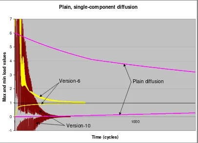
Figure 1 illustrates the differences in speed and behavior between our plain diffusion algorithm and our two algorithms for signal diffusion. For the sample runs shown in Figure 1, plain diffusion took15,816cycles to reach convergence, while the version-6 and version-10 algorithms took486and
361cycles, respectively. The instabilities that are characteristic of fast diffusion algorithms are evident from the sample runs in Figure 1. The largest and smallest values of the random start distribution were six and zero, respectively; the version-6 algorithm exhibited maximum load values as high as370, while the version-10 algorithms saw an extreme maximum value of160and an extreme minumum value of−180. We also note that the largest amount of load transferred over a link was0.0024for the plain diffusion algorithm; for each of the two signal diffusion algorithms, the largest value transferred over a link was about3. Thus we see a difference in this quantity by a factor of about 1000. In short: the “fast” one-component diffusion algorithms have oscillations, sometimes very high load/signal values at nodes, and sometimes very high transfers over the links.
3.4 Signal-aided diffusion
So far we have developed a single algorithm for slow diffusion of load (the plain diffusion algorithm) and two algorithms for the fast diffusion of signal (the version-6 and version-10 algorithms). We now present the practical details of our chemotaxis-inspired algorithm for load balancing: the signal-aided diffusion algorithm.
We recall our basic assumption that signal speed can be very high. Thus, for the signal, we are free to choose the fastest stable algorithm that we can find. After experimenting with half a dozen candidate algorithms, we arrived at the version-6 and the version-10 algorithms as our preferred candidates for fast signal diffusion algorithms.
Plain, single-component diffusion
Figure 1:Sample runs of the plain diffusion algorithm and the version-6 and version-10 diffusion algorithms. Largest and smallest values at the end of each cycle are plotted for the first 1500 cycles . All simulation runs used a random start distribution on a 10,000-node scale free topology.
to signal gradients. Our algorithm for Eq. (3) therefore incorporates the following two constraints. First, only nodes with more load than capacity are allowed to send to neighbors. Secondly, the total load sent must be less or equal to the difference between load and capacity of the sending node. The effect of these constraints is that once a node receives more load than capacity, it will maintain a load of at least capacity.
The main focus of our simulation experiments is to compare plain diffusion with signal-aided diffusion. It is therefore important to ensure that comparisons between the two be fair. We showed in section 2 that fairness means that the diffusion coefficient for load must be the same for both plain and signal-aided diffusion, i.e., we choose the same value forcandc3. Hence,candc3must be network-wide constants. We also recall thatcmust be smaller than the inverse degree of the most connected node in the topology.
We now have two load balancing algorithms for load that is restricted to move slowly. Plain diffusion simply sends out load in all directions independent of the current load distribution. Signal-aided diffusion, on the other hand, employs a fast-moving signal to guide load in directions that contain less load.
4
Performance
0
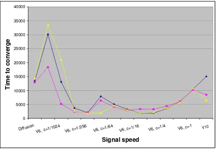
Figure 2: The effect of increasing signal diffusion speed on time to reach convergence for signal-aided load diffusion. Each of the three graphs corresponds to a different instance of our random start distribution. The convergence times for plain diffusion are plotted to the far left. All other plots show convergence times for signal-aided diffusion.
Our convergence time experiments aim at both comparing plain diffusion with signal-aided diffu-sion, and exploring the effect of different signal speeds on signal-aided diffusion performance. Recall that the Version 6 signal diffusion algorithm allows its speed to be altered by choosing different val-ues for the diffusion constantcdefault. The fastest signal diffusion speed is always obtained by our Version 10 algorithm. Version 6 withcdefault = 1gives the second fastest signal speed. Progressively slower signal speeds are then obtainded by halving the value of cdefault. We chose Version 6 with
cdefault= 1/2048as our slowest signal diffusion algorthm.
Figure 2 plots the time to reach convergence for a few sample runs, both for plain diffusion and for signal-aided diffusion with different signal speeds. Each of the three graphs in Figure 2 represents a set of sample runs sharing a particular instance of the random start distribution. Signal speed increases along the horizontal axis. Convergence times for plain diffusion are shown as the left-most plot of each graph. Note that, for this graph and for all subsequent plots showing performance, our results are based on only a small number of typical sample runs, and not on a statistical average over many runs, for each load speed. Also note that with respect to classes of topologies and start distributions, our experiments focus on only scale-free topologies and random start distributions. We revisit these issues in the future work section below and suggest that a wider range of experiment configurations is needed to provide stronger evidence that our algorithm behaves well in most situations.
0
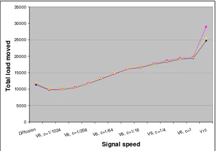
Figure 3: Total load moved to reach convergence as a function of signal speed. Each graph corresponds to a different instance of the random start distribution. Total load moved numbers for plain diffusion are plotted to the far left.
Several signal speeds produced reductions in convergence times of about 80%. (The shortest time to reach convergence for signal-aided diffusion was1795cycles; plain diffusion took about13,000
cycles to reach convergence.) Interestingly, the shortest convergence times were obtained when signal diffused at medium speeds. Signal-aided diffusion performed worse than plain diffusion when using our slowest signal speed (version 6 withcdefault= 1/2048).
Figure 3 shows the total load moved for the simulation runs depicted in Figure 2. It is interesting to see if the use of a guiding signal not only reduces the time to reach convergence but also leads to a reduction in the total load moved. Figure 3 tells us that most signal-aided runs appear to move more load in total than does plain diffusion. Also, we can observe a clear indication of an increase in total load moved with increasing signal speed. Only signal-aided runs with slower signal speeds, ie, those using the version-6 algorithm withcdefault <1/128, resulted in less load moved, and even then the reduction was modest compared to the increases experienced when using faster signal speeds.
0
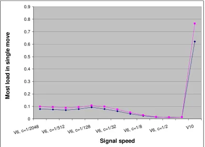
Figure 4:Largest load amount moved during any single cycle, over an entire simulation run, as a function of signal speed. Each graph represents a different instance of the random start distribution.
Though the results for largest single-step load amount moved are not as clear as the convergence time results, our tests suggest that performance gains are possible while still maintaining slow load movement. Also, it is worth noting that best results for the two-component algorithm, with version 6 for the signal, had a maximum link load moved that exceeded that for plain diffusion by a factor of only about 7. This may be contrasted with the factor 1000 increase for this same cost figure that we observed in the previous section (Figure 1), by increasing the single-component speed to the same value that signal uses in Figure 4. In other words (very roughly), by using chemotaxis instead of brute load speed, we obtain the same speed increase, but with much less penalty in maximum link load moved.
5
Nice properties
One of the main motivations for studying mechanisms from biology is that living systems exhibit “nice properties”: they are self-organizing, self-repairing, adaptive, etc. It is of course of great interest to inquire whether engineered systems also have these nice properties. In this section we offer a limited discussion of this kind of question for our chemotactic load balancing system.
0
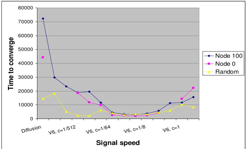
Figure 5:Sample runs showing time to reach convergence from different initial load distribution as a function of signal speed. Plain diffusion is plotted to the far left. Each graph represents a different start distribution. The three start distributions are: all load placed on a poorly connected node (node 100), all load placed on the best connected node (node 0), and random start distribution.
fact, we would argue that this type of insensitivity is in itself a kind of nice property. That is, insen-sitivity of performance to parameter values allows a self-organized system to find parameters giving good performance, without the necessity of fine tuning. Nevertheless we retain, as a goal for future work, the task of finding a satisfactory, decentralized method for tuning to a good value forcdefault.
Figure 2 also shows, in a limited way, another type of insensitivity. In this figure, it is clear that version-6 chemotaxis (for most speeds) and plain diffusion are each less sensitive to the particular ran-dom start distribution than is version-10 chemotaxis. Figure 5 gives us more insight into the question of this type of sensitivity. In the blue curve of this figure, the initial distribution consists of all the load (10,000 units) being placed at a very poorly connectd node (node 100). The red curve is generated from a start distribution with all load placed at the best connected node (node 0). Finally, the yellow curve comes from a random start distribution, like that used in Figure 2.
Hence Figure 5 shows results for a considerably larger variation of initial distribution than Fig-ure 2. We make three observations from FigFig-ure 5. First, version-10 chemotaxis is again more sensitive to initial distribution than is version-6 chemotaxis. Second, plain diffusion is highly sensitive to the initial load distribution. We see that the insensitivity and relatively good convergence times shown by plain diffusion for a random initial distribution are lost when we examine more extremely skewed start distributions. Finally, we feel that the insensitivity shown by the “good” range of version-6 chemo-taxis is remarkable: its convergence time is virtually indepedent of start distribution, even in the face of such extreme variations. While we do not have a detailed explanation for this nice property, we would claim that it merits the term “adaptivity”. In these words, we would say that (at least for this performance measure) version-6 chemotaxis is by far the most adaptive of the three systems studied.
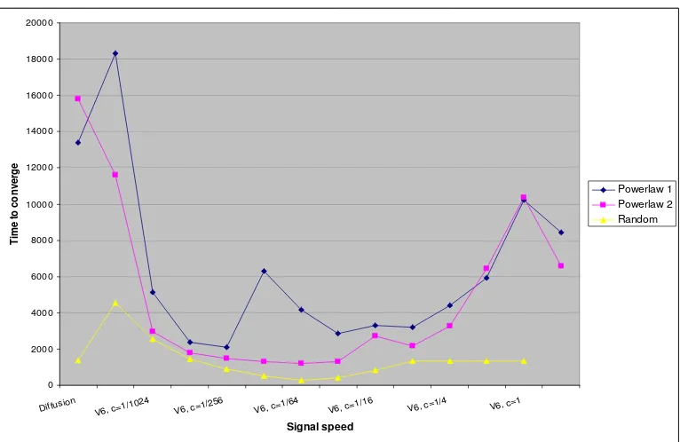
plat-0
Figure 6: Sample runs showing time to reach convergence on different topologies as a function of signal speeds. Plain diffusion plotted on the far left. Two graphs correspond to different instances of a powerlaw topology, the third graph corresponds to a random topology.
form [22], with a constant node degree (k= 20). Figure 6 shows some results for convergence time, comparing the random topology with the power-law topology. This figure thus shows sensitivity (or its inverse, adaptivity) to (rather large) topology variation. The two upper curves are for two distinct instances of the power-law topology, while the bottom (yellow) curve is for the random topology. Start distributions were random, generated for both topologies in the same way as outlined in section 4.
Our observations from this figure are roughly like those from Figure 5. That is: large sensitivity (poor adaptivity) for plain diffusion, and also for version-10 chemotaxis; and relatively low sensitivity for version-6 chemotaxis.
It is not so surprising that plain diffusion adapts poorly to changes in topology or initial distribu-tion. Plain diffusion is after all blind: it treats every “direction” on the network as equal. Intuition says that this blind approach should work best for (i) fairly uniform initial distributions, and (ii) a highly mixing topology such as the random topology; and Figures 5 and 6 are consistent with this. The news from these figures is then that our “smart” system is (at least, based on these tests) truly more adaptive than the blind system: it is only relatively weakly affected by the change from a random to a power-law topology, and virtually unaffected (in its best range) by changing from a fairly uniform start distribution to a highly skewed one.
6
Complex behavior
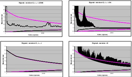
Signal: version 6, c = 1/2048
Figure 7:Sample runs showing approach to convergence (largest and smallest load values in the system under study) over time. Only the first 2500 cycles are plotted. Each sample run corresponds to a different signal speed; the chosen signal speeds are: version-6 withcdefault = 1/2048,cdefault = 1/64, andcdefault = 1in
addition to version-10. The time behavior of plain diffusion is included for reference in each plot. All runs use the same power-law topology and random start distribution.
the intuitive notions that we extract from the work of Cybenko [11]. We see that slow systems (plain diffusion in the figure) are stable, while the fastest stable one-component systems (version 10 in the figure) are close to instability. Version-6 one-component diffusion then represents an intermediate case.
Given the fact that the one-component diffusive system, when discretized, can give rise to oscilla-tions and instability, it is to be expected that the two-component system should do the same. In fact, our notion of two time scales corresponds, for continuous systems, to the notion of “stiff” coupled differential equations. It is known, for such systems, that coupling a “fast” system to a “slow”, fol-lowed by discretizing, can lead to oscillations, and even instability. Our chemotaxis system is such a system—but one for which there is no opportunity to adjust the size of the time step (the com-mon remedy for stiff systems). In this light, it is not surprising that the chemotaxis system exhibits oscillations. Nor is it surprising that the best performance, in terms of convergence, is obtained for intermediate (rather than maximal) values for the signal speed.
plunge. Hence, a weaker convergence criterion would rank this value forcdefaultconsiderably higher in performance.
The second plot (cdefault = 1/64) is taken from the “good” range of signal speeds. The approach to convergence is strikingly different from that in the first plot. In fact, the two systems are almost complementary: one (cdefault = 1/2048) shows a high rate of approach to convergence when far from convergence, and a low rate when close; while, for the other (cdefault= 1/64) the description is essentially reversed.
Yet another surprise is revealed by the third plot. Here we see behavior for the “fastest” (cdefault=
1) version-6 chemotaxis—and yet we see no oscillations whatsoever. Furthermore, the behavior is nearly identical to that of unaided diffusion, with c = 1/2500. We have no explanation for this behavior. Finally, moving to the fastest signal diffusion rule (version 10), we see in the fourth plot that the oscillations have returned.
This section is purely descriptive—we do not try to explain (yet) the complex behaviors seen here. The main points from this section are then that (i) the coupled system (even leaving out the unstable cases!) can exhibit highly complex behavior over time, on the way to convergence; and (ii) the nature of this complex behavior varies, as a function of signal speed, in a way that is in itself highly complex.
7
Discussion and Conclusions
In this paper, we have presented a biology-inspired mechanism for improving the performance of basic diffusion in load balancing. Diffusion is a widely studied approach that offers advantages of being simple, decentralized, and flexible. Our goal has been then to see if a more active mechanism, taken from biology, could give better results than the passive physics-inspired diffusion approach.
The mechanism that we borrow from biology is chemotaxis—a system in which diffusing chem-ical signals guide the movement of the bodies emitting them. We have allowed the load at nodes on a network to emit a signal, which follows a fast diffusion law for its motion. The motion of the load itself is then guided by gradients of signal. We have used repulsive chemotaxis—load moving down the gradient—to drive the load towards a uniform distribution. We have emphasized that chemo-taxis makes sense when there are two time scales present: the slow movement of the emitting bodies, coupled to the fast movement of the load. This idea may be technically useful when bandwidth con-straints prevent the load from diffusing rapidly, while signal (a few bytes) may not be subject to such constraints.
We have implemented a reference (plain diffusion) algorithm, and (after some experimentation) settled on two algorithms for fast diffusion of signal. One of our fast algorithms in fact allows for the continuous tuning of signal speed; hence we have been able to sample a wide range of signal speeds, always holding the load speed to a fixed (low) value.
Results of our tests show that chemotaxis can give a large improvement in rate of convergence over plain diffusion. These tests were performed on a scale-free topology with a random start distribution. The same tests show that the total load moved by chemotaxis is typically somewhat higher than that for plain diffusion (lower for some signal speeds, but up to a factor of two higher for others). Note that our results, though covering a wide range of signal speed values, are only based on a small number of runs. More work is needed to increase the number runs, each with a distinct instance of scale-free topology and random start distribution.
the links. We intend to examine this question in future work. (In fact, we have begun such studies, but cannot yet draw any definite conclusions.)
Our best algorithm for chemotaxis (“version 6”) has a tunable parameter (cdefault) which controls the signal speed. This is a global parameter. Hence another item for future work is to find satisfactory ways for the system itself to tunecdefaultto a good working value.
We note in this context that our version-6 chemotaxis rule gives good performance over a rather wide range of cdefault values. This kind of insensitivity is encouraging—it should make the task of decentralized self-tuning easier. Furthermore, we have observed other kinds of insensitivities for version 6: insensitivity to wide variations in start distribution, and to large differences in network topology. In fact, version-6 chemotaxis is clearly and unambiguously the best choice if this kind of insensitivity (or adaptivity) is important; both plain diffusion and version-10 chemotaxis showed much higher sensitivity to these two environmental perturbations.
The adaptivity that we see for version 6 is the kind of “nice property” that one hopes to achieve from decentralized, bio-inspired technological systems. We have noted the high adaptivity of version-6 chemotaxis. In particular, we find it remarkable that the convergence time for this rule, in the good range ofcdefaultvalues, is virtually unaffected by extreme variations in start distribution (Figure 5)— from fairly uniform, to the most disadvantageously skewed distribution possible. We note here that all three systems compared in this figure (plain diffusion, version 6, and version 10) are decentralized, flexible, ’swarm-intelligence-like’ systems. Hence, the argument that nice properties ’simply arise’ in such systems cannot help to explain the clear difference in adaptivity between these three. We leave the understanding of this also to future work.
Our chemotaxis system involves the coupling of two discrete dynamical systems, each with its own natural time scale (speed), and typically with a large difference between these two time scales. One does not expect smooth behavior from such systems. In fact, even the one-component (diffusive) system, because it is discrete, is subject to instabilities if it is too fast, and to oscillations when it is stable but near the instability threshold (Figure 1). The two-component system shows highly complex behavior (Figure 7). The good news is that simple precautionary rules, as reported in Section 3, can ensure that stable convergence can be reliably achieved, in spite of the complexity. However, an understanding of the complex behavior exhibited by our two-component system is lacking.
We have mentioned several topics for future work. Besides those mentioned, we plan on exploring other topologies; on collecting more systematic and quantitative results on nice properties such as adaptivity; and on seeking an understanding of the variations in adaptivity that we observe.
One further, outstanding, direction to take is to move the present approach towards practical ap-plication. The present work represents a proof of principle: that signalling can strongly enhance the convergence speed of a diffusive load balancing approach. We are interested in seeing whether this principle will survive in practice—for example, in large, dynamic systems such as peer-to-peer, where adaptivity is important, and central control is not practical.
8
Acknowledgments
We thank Niloy Ganguly for numerous helpful discussions. This work was partially supported by the Future & Emerging Technologies unit of the European Commission through Project BISON (IST-2001-38923).
References
[1] K. D. Devine, E. G. Boman, R. T. Heaphy, B. A. Hendrickson, J. D. Teresco, J. Faik, J. E. Flaherty, and L. G. Gervasio. New challenges in dynamic load balancing. Appl. Numer. Math., 52(2–3):133–152, 2005.
[2] A. Oram, editor. Peer-to-Peer: Harnessing the Benefits of a Disruptive Technology. O’Reilly & Associates, Mar. 2001.
[3] I. Foster and C. Kesselman, editors. The Grid: Blueprint for a Future Computing Infrastructure,. Morgan Kaufmann, 1999.
[4] E. Lee. Highly-available, scalable network storage. In 40th IEEE Computer Society
Interna-tional Conference (COMPCON95), page 397, 1995.
[5] Z. Palkova, B. Janderova, J. Gabriel, B. Zikanova, M. Pospisek, and J. Forstova. Ammona mediates communication between yeast colonies. Nature, 390:532–536, 1997.
[6] BISON. http://www.cs.unibo.it/bison/index.shtml.
[7] L. Benov and I. Fridovich. Escherichia coli exhibits negative chemotaxis in gradients of hydro-gen peroxide, hypochlorite, and N-chlorotaurine: Products of the respiratory burst of phagocytic cells. Proc. Nat. Acad. Sc. US, 93(10):4999–5002, 1996.
[8] J. C. Dallon, H. G. Othmer, C. v. Oss, A. Panfilov, P. Hogeweg, T. H¨ofer, and P. K. Maini. Models of Dictyostelium discoideum aggregation. In W. Alt, A. Deutsch, and G. Dunn, editors,
Dynamics of cell and tissue motion, pages 193–202. Birkh¨auser, Basel, 1997.
[9] P. N. Devreotes. Dictyostelium discoideum: A model system for cell-cell interactions in devel-opment. Science, 245:1054, 1989.
[10] Y. Jiang, H. Levine, and J. Glazier. Possible cooperation of differential adhesion and chemotaxis in mound formation of Dictyostelium. Biophys. J., 75:2615–2625, 1998.
[11] G. Cybenko. Dynamic load balancing for distributed memory multiprocessors. Journal of
Par-allel and Distributed Computing, 7:279–301, 1989.
[12] J. Boillat. Load balancing and poisson equation on a graph. Concurrency: Practice and
Experi-ence, 2:280–313, 1990.
[13] T. Decker, B. Monien, and R. Preis. Towards optimal load balancing topologies. Lecture Notes
in Computer Science, 1900:277–287, 2001.
[15] Y. F. Hu and R. J. Blake. An improved diffusion algorithm for dynamic load balancing. Parallel
Computing, 25:417–444, 1999.
[16] M. Jelasity, A. Montresor, and O. Babaoglu. A Modular Paradigm for Building Self-Organizing Peer-to-Peer Applications. In G. Di Marzo Serugendo, A. Karageorgos, O. F. Rana, and F. Zam-bonelli, editors, Engineering Self-Organising Systems: Nature-Inspired Approaches to Software
Engineering, number 2977 in Lecture Notes in Artificial Intelligence, pages 265–282.
Springer-Verlag, Apr. 2004.
[17] G. Karagiorgos and N. M. Missirlis. Accelerated diffusion algorithms for dynamic load balanc-ing. Inf. Process. Lett., 84(2):61–67, 2002.
[18] P. Sanders. On the efficiency of nearest neighbor load balancing for random loads. In Parcella
96, VII. International Workshop on Parallel Proccessing by Cellular Automata and Arrays, pages
120–127, 1996.
[19] R. Els¨asser and B. Monien. Diffusion load balancing in static and dynamic networks. In Proc.
Internat. Workshop on Ambient Intelligence Computing, pages 49–62, Dec. 2003.
[20] A. Deutsch, N. Ganguly, G. Canright, M. Jelasity, and K. Engø-Monsen. Models for advanced services in AHN, P2P Networks. Bison Deliverable, www.cs.unibo.it/bison/deliverables/D08.pdf, 2003.
[21] G. P. Jesi. Peersim howto: build a new protocol for the peersim simulation framework, November 2004.