Reframing the climate change challenge in
light of post-2000 emission trends
BY KEVIN ANDERSON AND ALICE BOWS*
Tyndall Centre for Climate Change Research, Mechanical, Civil and Aerospace Engineering, University of Manchester, PO Box 88, Manchester M60 1QD, UK
The 2007 Bali conference heard repeated calls for reductions in global greenhouse gas emissions of 50 per cent by 2050 to avoid exceeding the 28C threshold. While such endpoint targets dominate the policy agenda, they do not, in isolation, have a scientific basis and are likely to lead to dangerously misguided policies. To be scientifically credible, policy must be informed by an understanding of cumulative emissions and associated emission pathways. This analysis considers the implications of the 28C threshold and a range of post-peak emission reduction rates for global emission pathways and cumulative emission budgets. The paper examines whether empirical estimates of greenhouse gas emissions between 2000 and 2008, a period typically modelled within scenario studies, combined with short-term extrapolations of current emissions trends, significantly constrains the 2000–2100 emission pathways. The paper concludes that it is increasingly unlikely any global agreement will deliver the radical reversal in emission trends required for stabilization at 450 ppmv carbon dioxide equivalent (CO2e). Similarly, the current framing of climate change cannot be reconciled with the rates of mitigation necessary to stabilize at 550 ppmv CO2e and even an optimistic interpretation suggests stabilization much below 650 ppmv CO2e is improbable.
Keywords: emission scenarios; cumulative emissions; climate policy; energy; emission trends
1. Introduction
In the absence of global agreement on a metric for delineating dangerous from acceptable climate change, 28C has, almost by default, emerged as the principal focus of international and national policy.1 Moreover, within the scientific community, 28C has come to provide a benchmark temperature against which to consider atmospheric concentrations of greenhouse gases and emission reduction profiles. While it is legitimate to question whether temperature is an appropriate metric for representing climate change and, if it is, whether 28C is the appro-priate temperature (Tol 2007), this is not the purpose of this paper. Instead, the paper begins by considering the implications of the 28C threshold for global emission pathways, before proceeding to consider the implications of different emission pathways on stabilization concentrations and associated temperatures.
Published online
One contribution of 12 to a Theme Issue ‘Geoscale engineering to avert dangerous climate change’. * Author for correspondence ([email protected]).
1For example, in March 2007, European leaders reaffirmed their commitment to the 2
Although the policy realm generally focuses on the emissions profiles between 2000 and 2050, the scientific community tends to consider longer periods, typically up to and beyond 2100. By using a range of cumulative carbon budgets with differing degrees of carbon-cycle feedbacks, this paper assesses whether global emissions of greenhouse gases between 2000 and 2008, combined with short-term extrapolations of emission trends, significantly impact the 2008–2100 cumulative emission budget available, and hence emission pathways.
In brief, the paper combinescurrent greenhouse gas emissions data (including deforestation) with up-to-date emission trends and the latest scientific under-standing of the relationships between emissions and concentrations to consider three questions.
(i) Given a small set of emissions pathways from 2000 to a date where global emissions are assumed to peak (2015, 2020 and 2025), what emission reduction rates would be necessary to remain within the 2000–2100 cumulative emission budgets associated with atmospheric stabilization of carbon dioxide equivalent (CO2e) at 450 ppmv? The accompanying scenario set is hereafter referred to as ‘Anderson Bows 1’ (AB1).
(ii) Given the same pathways from 2000 to the 2020 emissions peak, what concentrations of CO2e are associated with subsequent annual emission reduction rates of 3, 5 and 7 per cent? The accompanying scenario set is hereafter referred to as ‘Anderson Bows 2’ (AB2).
(iii) What are the implications of the findings from (i) and (ii) for the current framing of the climate agenda more generally, and the appropriateness of the 28C threshold as the driver of mitigation and adaptation policy more specifically?
2. Analysis framing
(a) Correlating 28C with greenhouse gas concentration and carbon budgets What constitutes an acceptable temperature increase is a political rather than a scientific decision, though the former may be informed by science. By contrast, the correlation between temperature, atmospheric concentration of CO2e and anthropogenic cumulative emission budgets emerges, primarily, from our scientific understanding of how the climate functions.
Understanding current emission trends in particular and the links between global temperature changes and national emission budgets more generally (sometimes referred to as the ‘correlation trail’;Anderson & Bows 2007), is essential if policy is to be evidence based. Currently, national and international policies are dominated by long-term reduction targets with little regard for the cumulative carbon budget described by particular emission pathways. Within the UK, for example, while the government acknowledges the link between temperature and concentration, the principal focus of its policies is on reducing emissions by 60 per cent by 2050 (excluding international aviation and shipping; Bows & Anderson 2007). Closer examination of the UK’s relatively ‘mature’ climate change policy reveals a further inconsistency. Within many official documents 550 ppmv CO2e and 550 ppmv CO2 are used interchangeably,2 with the latter equating to approximately 615 ppmv CO2e (extrapolated from IPCC 2007a, topic guide 5, table 5.1); the policy repercussions of this scale of ambiguity are substantial.
Whether considering climate change from an international, national or regional perspective, it is essential that the associated policy debate be informed by the latest science on the ‘correlation trail’ from temperature and atmospheric concentrations of CO2e through to global carbon budgets and national emission pathways. Without such an informed debate, the scientific and policy uncertainties that unavoidably arise are exacerbated unnecessarily and significantly.
(b) Recent emissions data and science: impact on carbon budgets (i) Carbon-cycle feedbacks
The atmospheric concentration of CO2 depends not only on the quantity of emissions emitted into the atmosphere (natural and anthropogenic), but also on land use changes and the capacity of carbon sinks within the biosphere. As the atmospheric concentration of CO2 increases (at least within reasonable bounds), so there is a net increase in its take-up rate from the atmosphere by vegetation and the ocean. However, changes in rainfall and temperature in response to increased atmospheric greenhouse gas concentrations affect the absorptive capacity of natural sinks (Jones et al. 2006; Canadell et al. 2007; Le Que´re´
et al. 2007). While the complex and interactive nature of these effects leads to uncertainties with regard to the size of the carbon-cycle feedbacks (Cox et al. 2006), all models studied agree that a global mean temperature increase will reduce the biosphere’s ability to store carbon emissions over the time scales considered here (Friedlingstein et al. 2006). Consequently, pathways to stabilizing CO2 concentrations that include feedbacks have lower permissible emissions than those pathways that exclude such feedbacks. According to AR4, for example, with feedbacks included, stabilizing at 450 ppmv CO2e correlates with cumulative emissions some 27 per cent lower thanwithoutfeedbacks, over a 100-year period (IPCC 2007a, topic guide 5, p. 6). The impact of this latest science on the link between emissions and temperature is of sufficient scale to require the emission-reduction pathways associated with particular concen-trations and hence temperatures be revisited.
2For example, the RCEP uses CO
2e inRCEP (2000), whereas the Energy White Paper (DTI 2006)
(ii) Latest empirical emissions data
The current suites of emission scenarios informing the international and national climate change agenda seldom include empirical emissions data post-2000, choosing instead to model recent emissions; both the 2006 Stern Review (Stern 2006, p. 231) and the UK’s 2007 draft climate change bill (DEFRA 2007) illustrate this tendency. However, recent empirical data have shown global emissions to have risen at rates well in excess of those contained within these and many other emissions scenarios (Raupachet al. 2007). For example, while Stern assumes a mean annual CO2e emission growth between 2000 and 2006 of approximately 0.95 per cent, the growth rate calculated from the latest empirical data is closer to 2.4 per cent.3 Similarly, the UK’s draft climate change bill (DEFRA 2007) contains an emission pathway between 2000 and 2006 in which emissions fall, while over the same period the UK Government’s emission inventory suggests, at best, that emissions have been stable.
A further and important revision to recent emissions data relates to deforestation. Within many scenarios, including Stern, emissions resulting from deforestation are estimated to be in the region of 7.3 GtCO2 in 2000. However, recent data have suggested this to be an overestimate, with R. A. Houghton (2006, personal communication) having recently revised his earlier figure downward to 5.5 GtCO2.4 The impact of this reduction allied to the latest emission data reinforces the need to revisit emission pathways.
3. Scenario analysis
(a) Overview
The scenario analysis presented within this paper is for the basket of six greenhouse gases only and relies, principally, on the scientific understanding contained within AR4. The analysis does not take account of the following: — the radiative forcing impacts of aerosols and non-CO2 aviation emissions
(e.g. emissions of NOx in the upper troposphere, vapour trails and cirrus
formation);5 3CO
2data from the Carbon Dioxide Information Analysis Centre (CDIAC) including recent data
from G. Marland (2006, personal communication); non-CO2greenhouse gas data from the USA
Environmental Protection Agency (EPA 2006) including the projection for 2005, and assuming deforestation emissions in 2005 to be 5.5 GtCO2 (1.5 GtC), with a 0.4 per cent growth in the
preceding 5 years in line with data within the Global Forest Resources Assessment (FAO 2005).
4FAO (2005)contains rates of tropical deforestation for the 1990s revised downward from those in
the 2000 Global Forest Resources Assessment (FAO 2000; R. A. Houghton 2006, personal communication). An earlier estimate based on high-resolution satellite data over areas identified as ‘hot spots’ of deforestation, estimated the figure at nearer 3.7 GtCO2 (1 GtC) for 2000 (Achard
et al. 2004). It is Houghton’s more recent estimate that is used in this paper.
5There remains considerable uncertainty as to the actual level of radiative forcing associated
with aerosols, exacerbated by their relatively short residence times in the atmosphere and uncertainty as to future aerosol emission pathways (Cranmeret al. 2001; Andreaeet al. 2005). Similarly, there remain significant uncertainties as to the radiative forcing impact of non-CO2
emissions from aviation, particularly contrails and linear cirrus (e.g. Stordal et al. 2004;
— the most recent findings with respect to carbon sinks;6 — previously underestimated emission sources;7 and
— the implications of early emission peaks for ‘overshooting’ stabilization concentrations and the attendant risks of additional feedbacks.
While aerosols are most commonly associated with net global (or at least regional) cooling, the other factors outlined above are either net positive feedbacks or, as is the case for high peak-level emissions, increase the likelihood of net positive feedbacks. Consequently, the correlations between concentration and mitigation outlined in this analysis are, in time, liable to prove conservative. The scenarios are for CO2e emission pathways during the twenty-first century, with empirical data used for the opening years of the century (in contrast to modelled or ‘what if’ data). The full scenario sets (AB1 and AB2) comprise different combinations of the following: (i) emissions of CO2 from deforestation, (ii) emissions of non-CO2 greenhouse gases, and (iii) emissions of CO2 from energy and industrial processes.
For AB1
—Deforestation. Two low emission scenarios for the twenty-first century. —Non-CO2 greenhouse gases. Three scenarios peaking in 2015, 2020 and 2025
and subsequently reducing to 7.5 GtCO2e per year.
—Energy and process CO2. Three scenarios peaking in 2015, 2020 and 2025 and
subsequently reducing to maintain the total cumulative emissions for the twenty-first century within the AR4 450 ppmv CO2e range (with carbon-cycle feedbacks).
For AB2
—Deforestation. Two low emission scenarios for the twenty-first century. —Non-CO2 greenhouse gases. One scenario peaking in 2020 subsequently
reducing to 7.5 GtCO2e per year (as perAB1 with a 2020 peak).
—Energy and process CO2. Three scenarios, each following the same pathway to
a 2020 peak, but subsequently reducing at different rates to maintain total annual CO2e reductions of 3, 5 and 7 per cent.
The following sections detail the deforestation and non-CO2 greenhouse gas
emission scenarios used to derive the post-peakenergy and process CO2emission
scenarios and ultimately the total global CO2e scenarios for the twenty-first century.
(b) Deforestation emissions
A significant portion of the current global annual anthropogenic CO2 emissions are attributable to deforestation (in the region of 12–25%). However, carbon mitigation policy, particularly in OECD nations, tends to focus on those 6For example, and in particular, the reduced uptake of CO
2in the Southern Ocean (Raupachet al. 2007) and the potential impact of low level ozone on the uptake of CO2in vegetation (Cranmer
et al. 2001).
7For example, significant uncertainties in the emissions estimates for international shipping
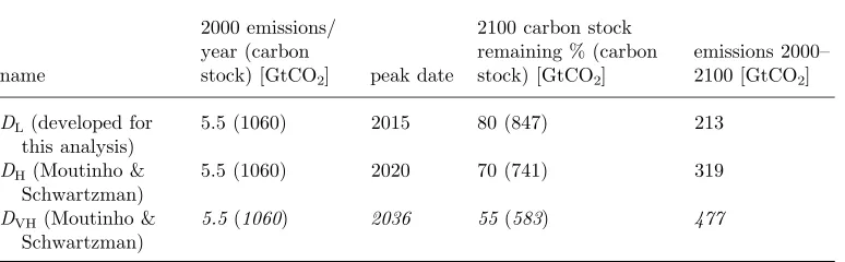
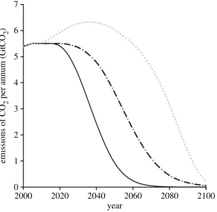
emissions from energy and industrial processes (hereafter referred to as energy and process emissions), with less direct regard for emissions arising from defore-station. While the relatively high levels of uncertainty associated with deforestation emissions make their inclusion in global mitigation scenarios problematic, the scale of emissions is such that they must be included. Within this paper two deforestation scenarios are developed; both assume climate change to be high on the political agenda and represent relatively optimistic reductions in the rate of, and hence the total emissions released from, deforestation.8 They both have a year 2000 baseline of 5.5 GtCO2, but post-2015 have different deforestation rates and hence different stocks of carbon remaining in 2100 (i.e. the amount of carbon stored in the remaining forest). The scenarios are illustrated numerically in table 1and graphically in figure 1.
The scenarios are dependent not only on the baseline but also on estimates of the change in forestry carbon stocks between 2000 and 2100. The stock values used in the scenarios are taken fromMoutinho & Schwartzman (2005)and based on their estimate of total forest carbon stock in 2000 of 1060 GtCO2. According to their assumptions, the carbon stock continues to be eroded at current rates until either 2012 or 2025, following which emissions from deforestation decline to zero by either 2100 or until they equate to 15 per cent of a particular nation’s forest stock (compared with 2000). They estimate two values for the carbon stocks, released as CO2 emissions by 2100 as 319 and 477 GtCO2. This implies that within their scenarios, either 70 or 55 per cent of total carbon stocks remain globally. Given that this paper and its accompanyingAB1andAB2scenarios are premised on climate change being high on the international agenda, Moutinho & Schwartzman’s55 per cent of total carbon stockvalue is considered too pessimistic within the context of this analysis, and although presented in figure 1, is not included in the analysis from this point onwards. Moreover, to allow for a more stringent curtailment of deforestation, the scenario developed for a 70 per cent stock-remaining estimate is complemented by one with 80 per cent remaining.
Table 1. Deforestation emission scenario summary for two scenarios used to build the subsequent full CO2e scenarios (deforestation low,DL; deforestation high,DH) and one for illustrative purposes
only (deforestation very high,DVH).
name
2000 emissions/ year (carbon
stock) [GtCO2] peak date
2100 carbon stock
5.5 (1060) 2015 80 (847) 213
DH(Moutinho &
Schwartzman)
5.5 (1060) 2020 70 (741) 319
DVH(Moutinho &
Schwartzman)
5.5(1060) 2036 55(583) 477
8While the scenarios are at least as optimistic as those underpinning, for example, the 2005 Forest
The DL and DH curves both assume no increase in deforestation rates from current levels, with DL beginning to drop from the peak level of 5.5 GtCO2, 5 years prior to DH. This, combined with the higher level of forestry, and hence carbon stock remaining in 2100, gives the DL curve a faster rate of reduction in deforestation than is the case for the DH curve (typically, 7.4 and 4.8% for DL and DH, respectively).9
(c) Non-CO2 greenhouse gas emissions
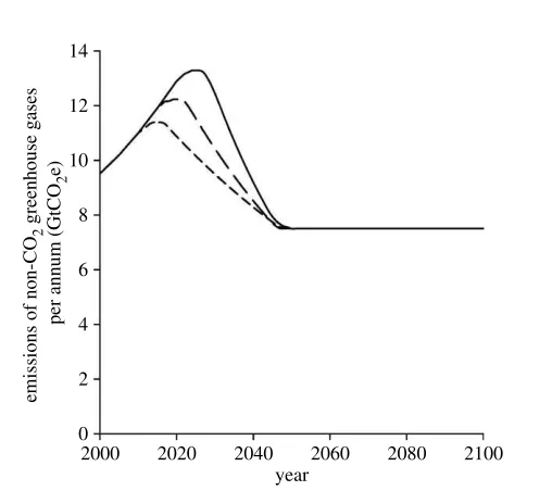
To estimate the percentage reductions required fromenergy and processCO2 emissions for both AB1 and AB2, it is necessary to consider a range of future emission scenarios for the non-CO2 greenhouse gases. Accordingly, three scenarios are developed assuming current US Environmental Protection Agency (EPA) estimates and projections of emissions from 2000 up to a range of peaking years, after which emissions are assumed to decline towards the same long-term stable level. All the scenarios represent a long-term halving in emission intensity, with the difference between them arising from the range of cumulative emissions associated with each of the peaking dates. The scenarios are illustrated numerically in table 2and graphically in figure 2.
Anthropogenic non-CO2greenhouse gas emissions are dominated by methane and nitrous oxide and, along with the other non-CO2 greenhouse gases, accounted for approximately 9.5 GtCO2e in 2000 (EPA 2006; similar figures are used within the Stern Review), equivalent to 23 per cent of global CO2e
2000 0 1 2 3 4
emissions of CO
2
per annum (GtCO
2
)
5 6 7
2020 2040 2060 year
2080 2100
Figure 1. Deforestation emission scenarios showing three CO2 emissions pathways based on
varying levels of carbon stocks remaining in 2100. Solid curve, 80% stock remaining; dot-dashed curve, 70% stock remaining; dotted curve, 55% stock remaining.
9
DLper cent change value is the mean for the period between 2030 and 2050, andDHis the mean
emissions. Understanding how this significant portion of emissions may change in the future is key to exploring the scope for future emissions reduction from all the greenhouse gases.
The three non-CO2 greenhouse gas scenarios presented here are broadly consistent with a global drive to alleviate climate change. The principal difference between the scenarios is the date at which emissions are assumed to peak, with the range chosen to match that for the total CO2e emissions, namely an early-action scenario where emissions peak in 2015, amid-actionpeak of 2020 and finally a late-actionpeak in 2025. All three scenarios have a growth rate from the year 2000 up until a few years prior to the peak, equivalent to that projected by theEPA (2006),10 and broadly in keeping with recent trend data. The scenarios all contain a smooth transition through the period of peak emissions and on to a pathway leading towards a post-2050 value of 7.5 GtCO2e. This value is again specifically chosen to
2000
Figure 2. Three non-CO2greenhouse gas emission scenarios with emission pathways peaking at
different years but all achieving the same residual level by 2050. Short dashed curve, early action; long dashed curve, mid-action; solid curve, late action.
Table 2. Non-CO2greenhouse gas emission scenario summary.
name
early action 9.5 2015 1.31 11.4 858
mid-action 9.5 2020 1.51 12.2 883
late action 9.5 2025 1.53 13.3 916
10EPA values for global warming potential of the basket of six gases are slightly different from
reflect a genuine global commitment to tackle climate change. It is approximately 25 per cent lower than the current level and consistent with a number of other 450 ppmv scenarios.11 Given that the majority of the non-CO2 greenhouse gas emissions are associated with food production, it is not possible, with our current understanding of the issues, to envisage how emissions could tend to zero while there remains a significant human population. The 7.5 GtCO2e figure used in this paper, assuming a global population in 2050 of 9 billion (thereafter remaining stable), is equivalent to approximately halving the emission intensity of current food production. While a reduction of this magnitude may be considered ambitious in a sector with little overall emission elasticity, such improvements are necessary if global CO2e concentrations are to be maintained within any reasonable bounds.
The non-CO2greenhouse gas scenarios have similar growth rates from 2000 to their respective peak values, and ultimately all have the same post-2050 emission level (7.5 GtCO2e). The rate of reduction in emissions from the respective peaks demonstrates the importance of timely action to curtail the current rise in annual emissions: the early-action scenario is required to reduce at 1.35 per cent per year, while themid-and late-action scenario values are at 2 and 3 per cent, respectively. Similarly,table 2and figure 2 demonstrate the importance for cumulative values of non-CO2greenhouse gas emissions not rising much higher than today and that the post-peak reduction rate achieves the long-term residual emission level as soon as is possible (7.5 GtCO2e by 2050). If the year in which emissions reach the residual level had been 2100 rather than 2050, the modest differences in cumulative emissions between theearly-, mid- and late-action scenarios would have been substantially increased. Given that the cumulative value of non-CO2greenhouse gas emissions is a significant proportion of total cumulative CO2e emissions, any delay in achieving the residual value would have significant implications for the reduction rate of energy and process CO2emissions necessary to meet theAB1andAB2criteria.
(d) CO2e emission scenarios for the twenty-first century
Having developed the deforestation and non-CO2 greenhouse gas scenarios, this section presents the complete greenhouse gas emission scenarios, AB1 and AB2, for the twenty-first century. The emissions released from the year 2000 until the peak dates are discussed here in relation to both AB1andAB2, before the post-peak scenarios for each of the scenario sets are presented.
(i) AB1 and AB2: emissions from 2000 to the peak years
By combining the deforestation and non-CO2 greenhouse gas scenarios with assumptions about energy and process CO2, scenarios for all greenhouse gas emissions up until the three peaking dates are developed. Energy and process CO2 emissions for the years 2000–2005 are taken from the Carbon Dioxide Information Analysis Centre (CDIAC), with estimates for 2006–2007 based on BP inventories (BP 2007). From 2007 to the three peaking dates of 2015 (early action), 2020 (mid-action) and 2025 (late-action) emissions of energy and process CO2grow at 3 per cent per year until 5 years prior to peaking. Beyond this point, emission growth gradually slows to zero at the peak year before reversing 11For example, in Stern (2006, p. 233), for both his 450 ppmv CO
2e and 500–450 ppmv
thereafter. The 3 per cent emission growth rate chosen for CO2 is broadly consistent with recent historical trends. Between 2000 and 2005, CDIAC data show a mean annual growth in energy and process CO2emissions of 3.2 per cent; this includes the slow growth years following the events of 11 September 2001.
(ii) AB1: emissions from peak years to 2100
From the peak years onwards,AB1(summarized intable 3) takes the approach that to remain within the bounds of a 450 ppmv CO2e stabilization target, the cumulative emissions between 2000 and 2100 must not exceed the range presented within the latest IPCC report in which carbon-cycle feedbacks are included (IPCC 2007b).
(iii) AB1 final scenarios
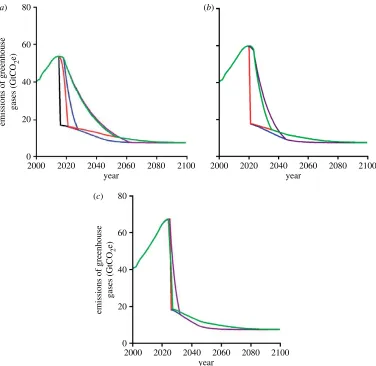
The emission pathways for the full greenhouse gasAB1scenarios from 2000 to 2100 are presented in figure 3. The plots comprise the earlier deforestation and non-CO2 greenhouse gas scenarios with growing energy and process CO2 emissions up to the peaking year, and all have total twenty-first century cumulative values of CO2e matching the 450 ppmv figures within AR4.
It is evident from the data underpinning figure 3 that 10 of the 18 proposed pathways cannot be quantitatively reconciled with the cumulative CO2e emissions budgets for 450 ppmv provided within AR4. Table 4 identifies the ‘impossible’ scenarios (including three with prolonged annual reduction rates greater than 15%) and illustrates the post-peak level of sustained emission reduction necessary to remain within budget.
(iv) AB1: implications for energy and process CO2
The constraints on the greenhouse gas emission pathways of achieving 450 ppmv CO2e render most of the AB1 scenarios impossible to achieve. Having established which scenarios are at least quantitatively possible and subtracting the respective non-CO2greenhouse gas and deforestation emissions, the energy and process emissions associated with each of the scenarios that remain feasible (figure 4) can be derived.
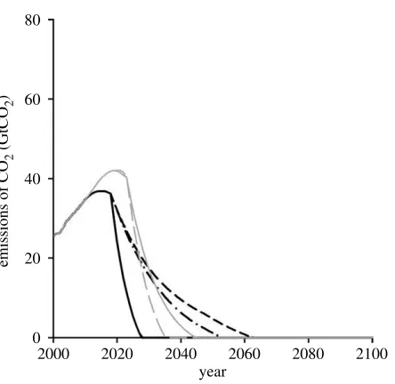
Figure 4 illustrates that complete decarbonization of the energy and process system is necessary by between 2027 and 2063, if the total greenhouse gas emissions are to remain within the IPCC’s 450 ppmv CO2e budgets. Moreover, in combination withtable 5, it is evident that the only meaningful opportunity for
Table 3. Summary of the core components of scenario setAB1.
characteristic 2015–2100 2020–2100 2025–2100
deforestationa DHandDL DHandDL DHandDL
non-CO2greenhouse gasesa early action mid-action late action
approximate peaking value [GtCO2e] 54 60 64
cumulative emissions [GtCO2e] IPCC
AR4
low: 1376 low: 1376 low: 1376 medium: 1798 medium: 1798 medium: 1798 high: 2202 high: 2202 high: 2202 2100 residual emissions [GtCO2e] 7.5 7.5 7.5
aDeforestation and non-CO
2000 0 20 40 60 80
2020 2040 2060 year
2080 2100
emissions of greenhouse
gases (GtCO
2
e)
2000 2020 2040 2060 year
2080 2100
(a) (b)
2000 0 20 40 60 80
2020 2040 2060 year
2080 2100
emissions of greenhouse
gases (GtCO
2
e)
(c)
Figure 3. Greenhouse gas emission scenarios forAB1with emissions peaking in (a) 2015, (b) 2020 and (c) 2025. Dark purple curve, lowDL; black curve, lowDH; blue curve, mediumDL; red curve,
mediumDH; light purple curve, highDL; green curve, highDH.
Table 4. Scenarios assessed in relation to their practical feasibility. (X denotes a scenario rejected on the basis of being quantitatively impossible or with prolonged percentage annual reduction rates greater than 15%. The percentage reductions given illustrate typical sustained annual emission reductions required to remain within budget.)
peak date
deforestationDL deforestationDH
low medium high low medium high
2015 X 13% 4% X X 4%
2020 X X 8% X X 11%
stabilizing at 450 ppmv CO2e occurs if the highest of the IPCC’s cumulative emissions range is used and if emissions peak by 2015.
(v) AB2: emissions from 2020(peak year) to 2100
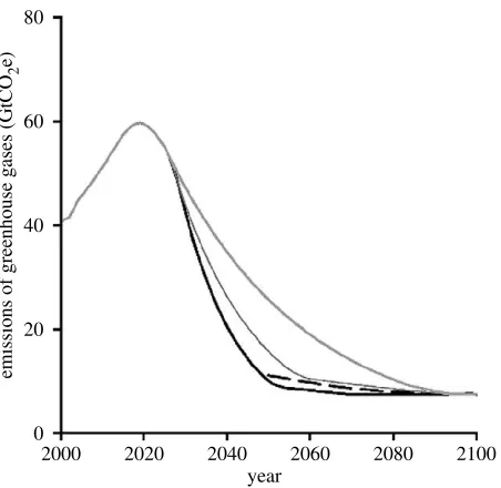
The AB2 scenario set complements the AB1 scenario set by exploring the implications for CO2e budgets of three post-peak annual emission reduction rates (3, 5 and 7%). Only one peaking year is considered within this analysis with 2020 chosen as arguably the most ‘realistic’ of the three dates in terms of both the ‘practicality’ of being achieved and of the respective scope for remaining within ‘reasonable’ bounds of CO2e concentrations. Table 6 summarizes the data underpinning figure 5.
2000 0 20 40 60
emissions of CO
2
(GtCO
2
)
80
2020 2040 2060 year
2080 2100
Figure 4. Energy and process CO2emissions derived by subtracting the non-CO2emissions and
deforestation emissions from the total greenhouse gas emissions over the period of 2000–2100, for theAB1scenarios. Black solid curve, 2015 peak mediumDL; black dashed curve, 2015 peak high
DL; dot-dashed curve, 2015 peak highDH; grey solid curve, 2020 peak highDL; grey dashed curve,
2020 peak highDH.
Table 5. Twenty-year sustained post-peak per cent reductions in energy and process CO2emissions
(from 5 years following the peak year). (X denotes a scenario rejected on the basis of being quantitatively impossible, with prolonged per cent annual reduction rates greater than 15% or scenarios where full decarbonization is necessary within 20 years.)
peak date
deforestationDL deforestationDH
low medium high low medium high
2015 X X w6% X X w8%
2020 X X X X X X
The pathways withinfigure 5equate to a range in cumulative CO2e emissions for 2000–2100 of 2.4 TtCO2e, 2.6 TtCO2e and 3 TtCO2e for 7, 5 and 3 per cent reductions, respectively. According to the cumulative emissions data contained within the Stern Review (Stern 2006: figure 8.1, p. 222), the first two values approximate to a CO2e concentration of approximately 550 ppmv with the latter being closer to 650 ppmv.
(vi) AB2: implications for energy and process CO2
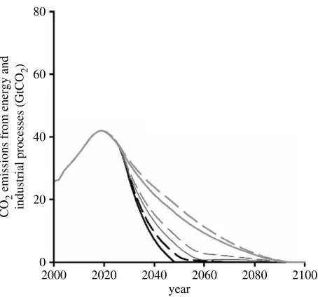
Having developed the total CO2e pathways for AB2, and given the deforestation and non-CO2 greenhouse gas emission scenarios outlined earlier, the associated energy and process CO2 scenarios can be derived (figure 6).
Table 7indicates typical post-peak annual reduction rates in energy and process CO2emissions for the families of 3, 5 and 7 per cent CO2e scenarios.
Table 6. Summary of the core components of theAB2scenarios.
characteristic 2020–2100
deforestationa DHandDL
non-CO2greenhouse gasesa mid-action
approximate peaking value [GtCO2e] 60
post-2020 CO2e reductions (%) 3, 5 and 7
2100 residual emissions [GtCO2e] 7.5
aDeforestation and non-CO
2greenhouse gas scenarios as intables 1and2.
2000 0 20 40 60
emissions of greenhouse gases (GtCO
2
e)
80
2020 2040 2060 year
2080 2100
Figure 5. Greenhouse gas emission scenarios peaking in 2020, with sustained percentage emission reductions of 3, 5 and 7%. The 3 and 5%DHscenarios are so similar to the 3 and 5%DLthat they are
hidden behind those profiles. Black solid curve, 7% reductionDL; black dashed curve, 7% reduction
DH; thin grey solid curve, 5% reductionDL; thin grey dashed curve (hidden), 5% reductionDH; thick
According to these results, the 3, 5 and 7 per cent CO2e annual reduction rates comprising the AB2 scenarios correspond with energy and process decarboniza-tion rates of 3–4, 6–7 and 9–12 per cent, respectively. While the latter two ranges correlate broadly with stabilization at 550 ppmv CO2e, the former, although arguably offering less unacceptable rates of reduction, correlates with stabilization nearer 650 ppmv CO2e.
4. Discussion
(a) AB1 scenarios
The AB1 scenarios presented here focus on 450 ppmv CO2e and can be broadly separated into three categories.
(i) Scenarios that quantitatively exceed the IPCC’s 450 ppmv CO2e budget range: this equates to 10 of the 18 scenarios. Scenarios in this category are quantitatively impossible.
2000 0 20 40 60
CO
2
emissions from ener
gy and
industrial processes (GtCO
2
)
80
2020 2040 2060 year
2080 2100
Figure 6. CO2 emissions derived by removing the non-CO2 greenhouse gas emissions and
deforestation emissions from the total greenhouse gas emissions over the period of 2000–2100 for theAB2scenarios. Black dashed curve, 7% reductionDL; black solid curve, 7% reductionDH; thin grey dashed curve, 5% reduction DL; thin grey solid curve, 5% reductionDH; thick grey dashed
curve, 3% reductionDL; thick grey solid curve, 3% reductionDH.
Table 7. Post-peak (2020) per cent reduction in energy and process CO2emissions.
annual reduction deforestationDL(%) deforestationDH(%)
total CO2e 3 5 7 3 5 7
(ii) Scenarios with current emission growth continuing until 2015, emissions peaking by 2020 and thereafter undergoing dramatic annual reductions of between 8 and 33 per cent. Scenarios in this category are, for the purpose of this paper, considered politically unacceptable.
(iii) Scenarios that, as early as 2010, break with current trends in emissions growth, with emissions subsequently peaking by 2015 and declining rapidly thereafter (approx. 4% per year). Scenarios in this category are discussed below.
For scenarios within category (iii) to be viable, it is necessary that the IPCC’s upper value for 450 ppmv cumulative emissions between 2000 and 2100 be correct. If, on the other hand, the IPCC’s mid- or low value turns out be more appropriate, category (iii) scenarios will either be politically unacceptable (i.e. above 8% per annum reduction) or quantitatively impossible.
However, even should the IPCC’s high level (‘optimistic’) value be correct, the accompanying 4 per cent per year reductions in CO2e emissions beginning in under a decade from today (i.e. by 2018) are unlikely to be politically acceptable without a sea change in the economic orthodoxy. The scale of this challenge is brought into sharp focus in relation to energy and process emissions. According to the analysis conducted in this paper, stabilizing at 450 ppmv requires, at least, global energy related emissions to peak by 2015, rapidly decline at 6–8 per cent per year between 2020 and 2040, and for full decarbonization sometime soon after 2050.
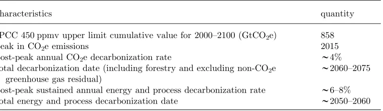
The characteristics of the resulting 450 ppmv scenario are summarized in
table 8. This assumes that the most optimistic of the IPCC’s range of cumulative emission values is broadly correct. While this analysis suggests stabilizing at 450 ppmv is theoretically possible, in the absence of an unprecedented step change in the global economic model and the rapid deployment of successful CO2 scrubbing technologies, 450 ppmv is no longer a viable stabilization concen-tration. The implications of this for climate change policy, particularly adaptation, are profound. The framing of climate change policy is typically informed by the 28C threshold; however, even stabilizing at 450 ppmv CO2e offers only a 46 per cent chance of not exceeding 28C (Meinshausen 2006). As a consequence, any further delay in global society beginning down a pathway towards 450 ppmv leaves 28C as an inappropriate and dangerously misleading mitigation and adaptation target.
Table 8. Summary of the core components of the 450 ppmv scenario considered theoretically possible within the constraints of the analysis and assuming the IPCC’s most ‘optimistic’ 450 ppmv CO2e cumulative value.
characteristics quantity
IPCC 450 ppmv upper limit cumulative value for 2000–2100 (GtCO2e) 858
peak in CO2e emissions 2015
post-peak annual CO2e decarbonization rate w4% total decarbonization date (including forestry and excluding non-CO2e
greenhouse gas residual)
w2060–2075
(b) AB2 scenarios
From the analysis underpinning theAB2scenarios, it is evident that the rates of emission reduction informing much of the climate change debate, particularly in relation to energy, correlate with higher stabilization concentrations than is generally recognized. The principal reason for this divergence arises, in the first instance, from the difference between empirical and modelled emissions data for post-2000. For example, in describing ‘[T]he Scale of the Challenge’ Stern’s ‘stabilization trajectories’ assume a mean annual emissions growth almost 1.5 per cent lower than was evident from the empirical data between 2000 and 2006. While the subsequent impact on cumulative emissions for this period is, in itself, significant, the substantive difference arises from short-term extrapolations of current trends. Stern’s range of peak emissions for 2015 are some 10 GtCO2e lower than would be the case if present trends continued out to 2010, with growth subsequently reducing to give a peak in emissions by 2015.12 This substantial divergence in emissions is exacerbated significantly as the peak date goes beyond 2015. If emissions were to peak by 2020 (as was assumed for theAB2scenarios), and again following a slowing in growth during the 5 years prior to the peaking date, emissions would, by 2020, be between 14 and 16 GtCO2e higher than Stern’s 2020 range. This difference alone equates to over a third of current global annual emissions, with knock-on implications for short- to medium-term cumulative emissions seriously constraining the viable range of long-term stabilization targets. While climate change is claimed to be a central issue within many policy dialogues, rarely are absolute annual carbon mitigation rates greater than 3 per cent considered viable. In addition, where mitigation polices are more developed, seldom do they include emissions from international shipping and aviation (Bows & Anderson 2007). Stern (2006, pp. 231) drew attention to historical precedents of reductions in carbon emissions, concluding that annual reductions of greater than 1 per cent have ‘been associated only with economic recession or upheaval’. For example, the collapse of the former Soviet Union’s economy brought about annual emission reductions of over 5 per cent for a decade. By contrast, France’s 40-fold increase in nuclear capacity in just 25 years and the UK’s ‘dash for gas’ in the 1990s both corresponded, respectively, with annual CO2 and greenhouse gas emission reductions of only 1 per cent (not including increasing emissions from international shipping and aviation). Set against this historical experience, the reduction rates contained within theAB2scenarios are without a structurally managed precedent. In all but one of the AB2 scenarios, the challenge faced with regard to total CO2e reductions is increased substantially when considered in relation to decarbonizing the energy and process systems. Despite the optimistic deforestation and non-CO2 greenhouse gas emission scenarios developed for this paper, the repercussions for energy and process emissions are extremely severe. Stabilization at 550 ppmv CO2e, around which much of Stern’s analysis
12Comparing values outlined in Stern (2006, p. 233) with those in AB1 and AB2 for 2015. In
addition, Stern envisages a global CO2e emissions increase of approximately 5 GtCO2e between
2000 and 2015 compared with provisional estimates for China alone of between 4.2 and 5.5 GtCO2e, extending up to 12.2 GtCO2e (T. Wang & J. Watson of the Sussex Energy Group
revolved, requires global energy and process emissions to peak by 2020 before beginning an annual decline of between 6 and 12 per cent; rates well in excess of those accompanying the economic collapse of the Soviet Union. Even for the 3 per cent CO2e reduction scenario (i.e. stabilization at 600–650 ppmv CO2e), the current rapid growth in energy and process CO2 emissions would need to cease by 2020 and begin reducing at between 3 and 4 per cent annually soon after.
It is important to note that for bothAB1andAB2scenarios, there is a risk of a transient overshoot of the ‘desired’ atmospheric concentration of greenhouse gases as a consequence of the rate of change in the emission pathway. Given that overshoot scenarios remain characterized by considerable uncertainty and are the subject of substantive ongoing research (e.g.Schneider & Mastrandrea 2005; Nusbaumer & Matsumoto 2008), they have not been addressed within either AB1 or AB2.
5. Conclusions
Given the assumptions outlined within this paper and accepting that it considers the basket of six gases only, incorporating both carbon-cycle feedbacks and the latest empirical emissions data into the analysis raises serious questions about the current framing of climate change policy. In the absence of the widespread deployment and successful application of geoengineering technologies (sometimes referred to as macro-engineering technologies) that remove and store atmos-pheric CO2, several headline conclusions arise from this analysis.
— If emissions peak in 2015, stabilization at450 ppmvCO2e requires subsequent annual reductions of 4 per cent in CO2e and 6.5 per cent in energy and process emissions.
— If emissions peak in 2020, stabilization at550 ppmvCO2e requires subsequent annual reductions of 6 per cent in CO2e and 9 per cent in energy and process emissions.
— If emissions peak in 2020, stabilization at650 ppmvCO2e requires subsequent annual reductions of 3 per cent in CO2e and 3.5 per cent in energy and process emissions.
These headlines are based on the range of cumulative emissions within IPCC AR4 (for 450 ppmv) and the Stern report (for 550 and 650 ppmv),13 with the accompanying rates of reduction representing the mid-values of the ranges discussed earlier. While for both the 550 and 650 ppmv pathways peak dates beyond 2020 would be possible, these would be at the expense of a significant increase in the already very high post-peak emission reduction rates.
It is increasingly unlikely that an early and explicit global climate change agreement or collective ad hoc national mitigation policies will deliver the urgent and dramatic reversal in emission trends necessary for stabilization at 450 ppmv CO2e. Similarly, the mainstream climate change agenda is far removed from the rates of mitigation necessary to stabilize at 550 ppmv CO2e. Given the reluctance, at virtually all levels, to openly engage with the unprecedented scale of both current emissions and their associated growth rates, even an optimistic interpretation of the current framing of climate change implies that stabilization much below 650 ppmv CO2e is improbable.
The analysis presented within this paper suggests that the rhetoric of 28C is subverting a meaningful, open and empirically informed dialogue on climate change. While it may be argued that 28C provides a reasonable guide to the appropriate scale of mitigation, it is a dangerously misleading basis for informing the adaptation agenda. In the absence of an almost immediate step change in mitigation (away from the current trend of 3% annual emission growth), adaptation would be much better guided by stabilization at 650 ppmv CO2e (i.e. approx. 48C).14 However, even this level of stabilization assumes rapid success in curtailing deforestation, an early reversal of current trends in non-CO2greenhouse gas emissions and urgent decarbonization of the global energy system.
Finally, the quantitative conclusions developed here are based on a global analysis. If, during the next two decades, transition economies, such as China, India and Brazil, and newly industrializing nations across Africa and elsewhere are not to have their economic growth stifled, their emissions of CO2e will inevitably rise. Given any meaningful global emission caps, the implications of this for the industrialized nations are bleak. Even atmospheric stabilization at 650 ppmv CO2e demands the majority of OECD nations begin to make draconian emission reductions within a decade. Such a situation is unprecedented for economically prosperous nations. Unless economic growth can be reconciled with unprecedented rates of decarbonization (in excess of 6% per year15), it is difficult to envisage anything other than a planned economic recession being compatible with stabilization at or below 650 ppmv CO2e.
Ultimately, the latest scientific understanding of climate change allied with current emission trends and a commitment to ‘limiting average global temperature increases to below 48C above pre-industrial levels’, demands a radical reframing16 of both the climate change agenda, and the economic characterization of contemporary society.
14Meinshausen (2006)estimates the mid-range probability of exceeding 4
8C at approximately 34 per cent for 600 ppmv and 40 per cent for 650 ppmv. Given this analysis has not factored in a range of other issues with likely net positive impacts, adapting for estimated impacts of at least48C appears wise.
15At 650 ppmv the range of global decarbonization rate is 3–4 per cent per year (table 7, columns 1
and 4). As OECD nations represent approximately 50 per cent of global emissions, and assuming continued CO2emission growth from non-OECD nations for the forthcoming two decades, the OECD
nations will need to compensate with considerably higher rates of emission reductions.
16This is not assumed desirable or otherwise, but is a conclusion of (i) the quantitative analysis
developed within the paper, (ii) the premise that stabilization in excess of 600–650 ppmv CO2e
References
Achard, F., Eva, H. D., Mayaux, P., Stibig, H.-J. & Belward, A. 2004 Improved estimates of net carbon emissions from land cover change in the tropics for the 1990s.Glob. Biogeochem. Cycles
18, GB2008. (doi:10.1029/2003GB002142)
Anderson, K. & Bows, A. 2007 A response to the draft climate change bill’s carbon reduction targets. Tyndall Centre briefing note 17, Tyndall Centre for Climate Change Research. See
http://www.tyndall.ac.uk/publications/briefing_notes/bn17.pdf.
Andreae, M. O., Jones, C. D. & Cox, P. M. 2005 Strong present-day aerosol cooling implies a hot future.Nature435, 1187–1190. (doi:10.1038/nature03671)
Bows, A. & Anderson, K. L. 2007 Policy clash: can projected aviation growth be reconciled with the UK Government’s 60% carbon-reduction target?Trans. Policy14, 103–110. (doi:10.1016/ j.tranpol.2006.10.002)
BP 2007 Statistical review of world energy 2007, British Petroleum. See http://www.bp.com/ liveassets/bp_internet/globalbp/globalbp_uk_english/reports_and_publications/statistical_ene rgy_review_2007/STAGING/local_assets/downloads/spreadsheets/statistical_review_full_rep ort_workbook_2007.xls.
Canadell, J. G.et al. 2007 From the cover: contributions to accelerating atmospheric CO2growth
from economic activity, carbon intensity, and efficiency of natural sinks.Proc. Natl Acad. Sci. USA104, 18 866–18 870. (doi:10.1073/pnas.0702737104)
Corbett, J. J. & Kohler, H. W. 2003 Updated emissions from ocean shipping.J. Geophys. Res.108, 4650. (doi:10.1029/2003JD003751)
Cox, P. M., Huntingford, C. & Jones, C. D. 2006 Conditions for sink-to-source transitions and runaway feedbacks from the land carbon-cycle. InAvoiding dangerous climate change(eds H. J. Schellnhuber, W. Cramer, N. Nakicenovic, T. Wigley & G. Yohe), pp. 155–161. Cambridge, UK: Cambridge University Press.
Cranmer, W.et al. 2001 Global response of terrestrial ecosystem structure and function to CO2and
climate change: results from six dynamic global vegetation models. Glob. Change Biol. 7, 357–373. (doi:10.1046/j.1365-2486.2001.00383.x)
DEFRA 2006 Climate change: the UK Programme 2006. Norwich, UK: HMSO, Department of Food and Rural Affairs.
DEFRA 2007Draft climate change bill. London, UK: HMSO, Department of Food and Rural Affairs. DTI 2006Our energy challenge: securing clean, affordable energy for the long term. London, UK:
HMSO, Department of Trade and Industry.
EPA 2006 Global anthropogenic non-CO2 greenhouse gas emissions: 1990–2020. Office of
Atmospheric Programs, Climate Change Division, USA Environmental Protection Agency. European Commission 2007Limiting global climate change to 2 degrees Celsius: the way ahead for
2020 and beyond. Brussels, Belgium: Commission of the European Communities.
Eyring, V., Ko¨hler, H. W., van Aardenne, J. & Lauer, A. 2005 Emissions from international shipping: 1. The last 50 years.J. Geophys. Res.110, D17305. (doi:10.1029/2004JD005619) FAO 2000 Global forest resources assessment 2000. FAO forestry paper no. 140. Food and
Agriculture Organisation of the United Nations, Rome.
FAO 2005 Global forest resources assessment 2005. Global synthesis FAO forestry paper no. 124. Food and Agriculture Organisation of the United Nations, Rome.
Friedlingstein, P. et al. 2006 Climate-carbon-cycle feedback analysis, results from the C4MIP model intercomparison.J. Clim.19, 3337–3353. (doi:10.1175/JCL13800.1)
IPCC 1996 Climate change 1995: the science of climate change. Contribution of working group 1 to the second assessment report of the Intergovernmental Panel on Climate Change.
IPCC 2007a Climate change 2007: synthesis report. Fourth assessment report of the Intergovernmental Panel on Climate Change.
Jones, C. D., Cox, P. M. & Huntingford, C. 2006 Impact of climate-carbon-cycle feedbacks on emissions scenarios to achieve stabilisation. In Avoiding dangerous climate change (eds H. J. Schellnhuber, W. Cramer, N. Nakicenovic, T. Wigley & G. Yohe), pp. 323–331. Cambridge, UK: Cambridge University Press.
Le Que´re´, C.et al. 2007 Saturation of the Southern Ocean CO2sink due to recent climate change.
Science316, 1735–1738. (doi:10.1126/science.1136188)
Mannstein, H. & Schumann, U. 2005 Aircraft induced contrail cirrus over Europe.Meteorologische Zeitschrift14, 549–554. (doi:10.1127/0941-2948/2005/0058)
Meinshausen, M. 2006 What does a 2C target mean for greenhouse gas concentrations? A brief analysis based on multi-gas emission pathways and several climate sensitivity uncertainty estimates. In Avoiding dangerous climate change (eds H. J. Schellnhuber, W. Cramer, N. Nakicenovic, T. Wigley & G. Yohe), pp. 253–279. Cambridge, UK: Cambridge University Press.
Moutinho, P. & Schwartzman, S. (eds) 2005 Tropical deforestation and climate change. Bele´m, Brazil: Amazon Institute for Environmental Research.
Nusbaumer, J. & Matsumoto, K. 2008 Climate and carbon-cycle changes under the overshoot scenario.Glob. Planet. Change62, 164–172. (doi:10.1016/j.gloplacha.2008.01.002)
Raupach, M. R., Marland, G., Ciais, P., Le Quere, C., Canadell, J. G., Klepper, G. & Field, C. B. 2007 Global and regional drivers of accelerating CO2emissions.Proc. Natl Acad. Sci. USA104,
10 288–10 293. (doi:10.1073/pnas.0700609104)
RCEP 2000 Energy—the changing climate, 22nd report, CM 4749. The Stationery Office, London. Schneider, S. H. & Mastrandrea, M. D. 2005 Inaugural article: probabilistic assessment of “dangerous” climate change and emissions pathways. Proc. Natl Acad. Sci. USA 102, 15 728–15 735. (doi:10.1073/pnas.0506356102)
Stern, N. 2006Stern review on the economics of climate change. Cambridge, UK: Her Majesty’s Treasury, Cambridge University Press.
Stordal, F., Myhre, G., Arlander, W., Svendby, T., Stordal, E. J. G., Rossow, W. B. & Lee, D. S. 2004 Is there a trend in cirrus cloud cover due to aircraft traffic?Atmos. Chem. Phys. Discuss.4, 6473–6501.