HOW TRAVEL DEMAND AFFECTS DETECTION OF NON-RECURRENT TRAFFIC
CONGESTION ON URBAN ROAD NETWORKS
B. Anbaroglu a*, B. Heydecker b, T. Cheng c
a Hacettepe University, Dept. of Geomatics Engineering, 06800, Beytepe, Ankara, Turkey - [email protected] b Centre for Transport Studies, Civil, Environmental and Geomatic Engineering, University College London, Gower Street, London,
WC1E 6BT UK - [email protected]
c SpaceTimeLab, Civil, Environmental and Geomatic Engineering, University College London, Gower Street, London, WC1E 6BT
UK - [email protected]
Commission II, WG II/3
KEY WORDS: Non-recurrent congestion, space-time clustering, space-time scan statistics, urban road network, travel demand
ABSTRACT:
Occurrence of non-recurrent traffic congestion hinders the economic activity of a city, as travellers could miss appointments or be late for work or important meetings. Similarly, for shippers, unexpected delays may disrupt just-in-time delivery and manufacturing processes, which could lose them payment. Consequently, research on non-recurrent congestion detection on urban road networks has recently gained attention. By analysing large amounts of traffic data collected on a daily basis, traffic operation centres can improve their methods to detect non-recurrent congestion rapidly and then revise their existing plans to mitigate its effects. Space-time clusters of high link journey time estimates correspond to non-recurrent congestion events. Existing research, however, has not considered the effect of travel demand on the effectiveness of non-recurrent congestion detection methods. Therefore, this paper investigates how travel demand affects detection of non-recurrent traffic congestion detection on urban road networks. Travel demand has been classified into three categories as low, normal and high. The experiments are carried out on London’s urban road network, and the results demonstrate the necessity to adjust the relative importance of the component evaluation criteria depending on the travel demand level.
1. INTRODUCTION
Traffic congestion is one of the most haunting issues of a developed urban environment as it has a substantial impact on society and nature (Beevers and Carslaw, 2005; Goodwin, 2004). Even though traffic congestion is intrinsically linked with the economic success of a city; no one would be willing to waste time and money due to a congestion event. In addition, urban road networks could barely increase traffic capacity by widening existing roads or building new roads due to the existing infrastructure. Even if the existing infrastructure allows for new developments, implementation of such solutions is usually cost prohibitive and requires elaborate planning. Consequently, improving traffic capacity is not a sustainable strategy to manage traffic congestion on the long term (National Research Council, 1994).
Urban road networks face with two main types of traffic congestion: recurrent and non-recurrent. Recurrent congestion exhibits a daily pattern and it is observed at morning or afternoon peak periods. Location and duration of a recurrent-congestion event is usually known by regular commuters and traffic operators. Excess travel demand, inadequate traffic capacity or poor signal control are the main reasons of recurrent congestion (Han and May, 1989). On the other hand, Non-Recurrent Congestion events (NRCs) are mainly caused by unexpected events like traffic accidents or vehicle breakdowns; and planned events like engineering works or special events such as football matches or concerts (FHWA, 2012; Kwon et al., 2006). An NRC event can occur at any time of day, and its location and duration usually depends on the travel demand, as well as the local conditions of the road network and traffic capacity. Amongst
* Corresponding author
these factors, focusing on travel demand is relatively more important, as traffic operation centres need to develop action plans based on the travel demand level.
Variations in travel demand affect many important indicators such as travel time reliability, economic success of a city and the structuring of policies such as congestion charge (Yang and Bell, 1997). There is a growing research interest to detect NRCs on an urban road networks; yet, the variation of travel demand on the effectiveness of such approaches has not been investigated so far (Anbaroğlu et al., 2015). Therefore, this paper aims to investigate how different travel demand levels affect the performance of NRC detection methods.
2. LITERATURE REVIEW
Understanding the formation and propagation of traffic congestion has taken the interest of researchers for decades. Previous studies on congestion detection have focused on motorways/freeways, which are not subject to interruptions due to traffic lights or pedestrian crossings. Uninterrupted traffic flow on motorways allowed scientists to develop physical models to explain the formation and development of traffic congestion as a ‘cluster of densely moving vehicles’ (Kerner and Konhäuser, 1994; Treiber et al., 2000). Investigation of the characteristics of traffic congestion on urban road networks remained a challenge due to difficulty in modelling irregular interruptions such as traffic lights.
The advancement of sensor technology and communication networks allows traffic operation centres to collect vast amounts
of traffic data on a daily basis (Chang et al., 2004). Investigation of such rich datasets might eventually overcome the difficulties of analysing urban road networks (Geroliminis and Sun, 2011). A prominent example is the Link Journey Time (LJT) data, in which an LJT is an approximation of the journey time through a link at an established time interval. Traffic operation centres often rely on LJTs to assess network performance, due to its suitability for network-wide analysis (Hall, 2001). Estimation of an LJT requires the calculation of a vehicle’s travel time through a link, which is obtained by matching the readings of automatic number plate recognition cameras (Robinson and Polak, 2006).
Modelling the statistical distribution of LJTs has been an attractive research area for decades due to its linkage with travel time reliability (Hollander and Liu, 2008; Wardrop, 1952). However, what is meant by “distribution of travel time” might vary depending on the context. For example, Arezoumandi (2011) and Susilawati et al. (2011) attempt to find a distribution to characterise the travel times on a link, regardless of the temporal variations within a day. On the other hand, Polus (1979) considers two time periods (i.e. to and from work trips). Secondly, different road characteristics may result in different outcomes. For example, link lengths have shown a distinctive effect (e.g. making the distribution bimodal) on the distribution of travel times (Susilawati et al., 2011). Furthermore, only few studies mention the data cleaning procedure, which might have a substantial impact on the distribution of LJTs (Anbaroğlu et al., 2015).
Investigating the linkage between travel demand and LJTs is also an exciting research endeavour (Gronau, 1970). Commuters usually aim to reduce their travel times as well as improve the predictability of their journeys –both of which directly relate to travel demand (Carrion and Levinson, 2012). For instance, the occurrence of a tube strike would increase the demand for ground transportation modes, which in turn increase the LJTs (Moylan et al., 2016; Tsapakis et al., 2013). Understanding how the road network would operate under unusually high travel demand levels would be useful when developing contingency plans. Similarly, a thorough understanding of travel times for low travel demand levels is also necessary when time-critical operations (e.g. ambulance dispatch) are to be assessed (Schmid and Doerner, 2010).
3. SPACE-TIME CLUSTERING TO DETECT NRCS
This paper builds upon the two recent NRC detection methods as described in Anbaroğlu et al. (2015). These methods aim to capture the heterogeneous nature of an urban road network, due to variations in link lengths and data quality, by modelling link journey time estimates with a lognormal distribution. Percentile based NRC detection relies on the percentile values of the estimated LJTs to detect NRCs. Space-time scan statistics (STSS) based NRC detection relies on a statistical model to detect statistically significant clusters of high LJTs.
The developed methodology relies on several inputs. Adjacency matrix (M) is a binary matrix defining the connectivity of the links. Congestion factor (c) is a real-valued number multiplied with the expected LJTs to determine the threshold to identify whether an LJT is excessive. Last, NRCs are detected on a given date of analysis.
3.1 Percentile based NRC Detection
A percentile is a measure indicating the value below which a given percentage of observations in a group of observations fall.
For example, the 95th percentile of an LJT would indicate that the 95% of the estimated LJTs are indeed below that value. There are different ways to calculate a given percentile value. In this paper, we rely on the percent point function method, as it considers the statistical distribution of LJTs (Pu, 2011). Consequently, the percentiles of an estimated LJT are determined as shown in equation (1).
� � = exp � + �Φ− � (1)
where p is the cumulative probability, Φ− � is the percent point function of the standard normal distribution function, μ and
σ are the mean and standard deviation of the underlying normal distribution, respectively. The value of Φ− � could be obtained easily given p. For example, when p = 0.5, Φ− � would be zero; hence, G(0.5) = exp(μ), which is the median of the lognormal distribution.
The aforementioned process to calculate the πth percentile value (π = 100p) of an LJT is conducted for all a ∈ A and t ∈ {1, 2, ... , T}, where A and T denote the set of links and the total number of LJTs within the analysis interval respectively. Specifically, G(p) is calculated for |A|.T times for a given value of π. Thereon, an estimated LJT on link a time interval t, � , is considered to belong to an NRC if it is greater than its πth percentile value. Formally, � belongs to an NRC if � > �� , where �� denotes the πth percentile value of link a at time interval t.
Those LJTs that are higher than their πth percentile values and spatio-temporally overlap with each other are clustered to detect NRCs. Two LJTs spatio-temporally overlap with each other if they either occur on the same link at adjacent time intervals (i.e. � and � + ) or occur on adjacent links at the same time interval (i.e. � and � , where � , = ). This procedure of clustering spatio-temporally overlapping LJTs is repeated until all the LJTs that are higher than their πth percentile value are included within an NRC.
3.2 STSS based NRC Detection
Space-time scan statistics (STSS) is a state-of-the-art cluster detection method (Patil and Taillie, 2004). This statistical method is modified for the purpose of NRC detection, and consists of four steps (Anbaroğlu et al., 2015). First, space–time regions (STRs) are generated which requires two inputs: maximum spatial window size (ρ) and maximum temporal window size (τ). Second, the likelihood ratio function (Ƒ) is determined by considering the distribution of LJTs. The whole analysis period is scanned with overlapping STRs and their likelihood ratio scores are calculated. Third, significant STRs are determined by comparing the likelihood ratio scores of the observed data with the ones obtained from the replications. Finally, significant STRs are clustered to detect NRCs.
A space-time region (STR) is the aggregation of spatial regions in time, where links correspond to the spatial regions. An NRC may span several links and its duration cannot be known a prior. In order to detect any NRC regardless of the number of links that it contains or its duration, it is necessary to scan an entire study area with overlapping STRs whose size and location varies. To generate all possible STRs, two parameters should be determined: maximum spatial window size (ρ) and maximum temporal window size (τ). However, scanning a large spatial area containing hundreds of regions is computationally unfeasible (Neill and Moore, 2004). Therefore, it is necessary to reduce the number of STRs and this is accomplished with the following two adjustments. First, only those STRs whose individual LJTs are
excessive are evaluated. Second, spatial regions are created by only considering the link itself and its first-order adjacencies.
The likelihood ratio function of an STR s whose individual LJTs are lognormally distributed is stated in equation (2) (Anbaroğlu et al., 2015). where STR denotes the set of all STRs.
The third step, determining significant STRs, requires a number of replications of the dataset. The replications are generated based on the null hypothesis that no NRC had occurred during the analysis period. Each LJT is replicated based on its distribution. Having obtained the replications, STRs are used to scan these replications and their likelihood ratio scores are obtained. The highest likelihood ratio score of each replication is recorded. Finally, the observed likelihood ratio scores are compared with the distribution of highest likelihood ratio scores of the replications to determine significant STRs.
The last step of STSS based NRC detection is the clustering of significant STRs. When generating STRs only the link itself and its first-order adjacencies are considered; however, an NRC may span many links. In order to detect such NRCs, spatio-temporally overlapping significant STRs are clustered. Clustering significant STRs has a similar procedure to the one described in Percentile based NRC detection. This is because an STR is a group of LJTs, and all the LJTs that belong to a statistically significant STR are considered to belong to an NRC. Thereon, spatio-temporally overlapping LJTs could be clustered to detect NRCs.
3.3 Evaluation of NRC Detection Methods
Both of the NRC detection methods would detect a number of NRCs, but the detected NRCs would be different depending on the method and its parameters. For example, different π values in Percentile based NRC detection would lead to different NRCs. Similarly, different maximum spatial and temporal window size values in STSS would lead to, again, different NRCs. The main issue is to determine, which one of these different outcomes resemble the reality the most.
A conceivable way would be to compare the detected NRCs with the real NRCs, and assess to what extent they match with each other. However, knowing the true spatial and temporal extent of all NRCs, even for a single day, govern remarkable challenges. Therefore, two complementary evaluation criteria have been proposed: high-confidence episodes and the Localisation Index (Anbaroglu et al., 2014).
A ‘high-confidence’ episode is an NRC event on a link that lasts for a minimum duration during which all LJTs are excessive. The detected NRCs are compared with respect to the high-confidence episodes to obtain two measures. False Alarm Rate (FAR) is the proportion of all LJTs that are enclosed within an NRC but a high-confidence episode to all LJTs enclosed by the NRCs. False Negative Rate (FNR) is the proportion of all LJTs that are enclosed within a high-confidence episode but the detected NRCs to all LJTs enclosed by the high-confidence episodes. Of these
two measures, FNR is the critical one as it determines the proportion of missed high-confidence episodes.
The Localisation Index (LI) assesses to what extent an NRC detection method considered day-to-day variations in traffic to belong to an NRC. For example, a liberal NRC detection method may be very good at detecting high-confidence episodes; however, it may also lead to detecting large NRCs that do not necessarily represent the reality. In order to penalise such liberal methods, an NRC detection method should be able to produce compact NRCs. In this way, the detected NRCs could be associated with real-life events, such as incidents or engineering works. The ‘Localisation Index’ is an evaluation criterion that quantifies the extent to which the detected NRCs consist of link groups that are adjacent throughout their life-time. If only a single link group (i.e. a number of links all of which form a single connected component) occurs through-out the life time of an NRC, then its LI value would be one, which is the best score for LI. This step is repeated for all the detected NRCs, and the highest LI value would be the LI of the model.
Once the FNR and LI are determined; these complementary criteria has to be combined into one so that a researcher could decide on the best performing NRC detection model. Multi-Attribute Decision Making (MADM) provides the necessary theoretical background to perform this task. There are many methods of MADM; however, in this paper we rely on the Weighted Product Model (WPM) to combine the two criteria into a single measure (Triantaphyllou and Mann, 1989). The main included. The Final Score (FS) of WPM is calculated as shown in equation (3). criterion of Kth and Lth NRC detection models respectively, and �� is the weight (i.e. the relative importance) of criterion j. Having determined all Final Score values, the best model is the one that has the smallest Final Score, because the smaller the values of both of the criteria, �∗ and the LI, the better the NRC detection model. Once all NRC detection models are compared with one another, they can be ranked based on their Final Score values.
4. RESULTS
The proposed NRC detection methodology has been applied to London’s urban road network. The road network consists of 424 links and LJTs are estimated every five minutes. The analysis has been conducted between 07:00 and 19:00, as this time interval covers the AM/Inter/PM peak periods in London (TfL, 2010). Therefore, for a given link there would be 145 LJTs (12 hr × 12 LJTs/hour + 1, since the analysis period is inclusive of 07:00 and 19:00).
The investigation is carried out on three different travel demand levels, bank holidays, normal days and tube strikes corresponding to low, normal and high travel demand for the year 2010. The days that are included within these travel demand levels are illustrated in Table 1.
Bank Holidays (Low)
1 January , 2 April, 5 April, 3 May, 31 May, 30 August, 27 December, 28 December.
Normal Days (Normal)
Weekdays of October except 4 October on which a tube strike occurred.
Tube Strikes (High)
7 September, 4 October, 3 November, 29 November.
Table 1. The investigated days on three different demand levels
Traffic operators commonly use expected LJTs for road network performance monitoring. This paper uses the expected LJTs that are used in Transport for London (TfL). In this way, there would be consistency between our analysis and the practice. As aforementioned, running an unmodified STSS model is a cost-prohibitive in terms of computational time. Therefore, this paper considers only excessive LJTs, which are 20% higher than their expected values (i.e. c = 1.2). The main reason for us to rely on such excessive LJTs is the practical guidelines, in which TfL considers a link to have ‘minimal congestion’ whenever estimated LJTs are 20% higher than their expected values (TfL, 2010).
The other parameters of STSS based NRC detection are; the maximum spatial (ρ) and temporal window sizes (τ). The maximum spatial window size is varied between one and three; as our empirical analysis suggest that the combined effect of links do not have a substantial effect on the detected NRCs for STRs containing three or more adjacent links. The maximum temporal window size is varied between one and six, as 30 minutes is sufficiently long enough for an NRC to develop. Number of replications is decided to be 99, so that the lowest p-value would be 0.01. The significance level is determined to be 0.05, so that whenever the p-value of an STR is less than 0.05 it would be considered to be significant. On the other hand, the only parameter of Percentile based NRC detection, π, is varied between 75 and 95, as this range would correspond to the unusually high LJTs (Anbaroğlu et al., 2015).
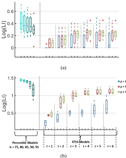
In order to provide a better understanding of the NRC detection methods, the boxplot of LI values for different models are illustrated in Figure 1 for low and high travel demand levels (i.e. bank holidays and tube strikes respectively). The boxplot is shown in log-scale in order to improve the legibility of the results.
The common outcome is that STSS models are more conservative in detecting NRCs; hence, resulted in better performance regarding the LI. The lower the spatial and temporal window sizes, the more conservative STSS models become. The results also suggest to liberalise an STSS model by increasing its temporal window size rather than spatial window size. As an expected outcome, as the π value in Percentile based NRC detection increases the method becomes more conservative, since the � � > �� would decrease.
(a)
(b)
Figure 1. Variations of Localisation Index values of different NRC detection models on bank holidays (a) and tube strikes (b)
On the other hand, STSS based NRC detection performs poorer with respect to the detection of high-confidence episodes. For London’s urban road network, empirical analyses demonstrate that a high-confidence episode occurs whenever the estimated LJTs are at least 40% higher than their expected values for at least a minimum duration of 25 minutes (Anbaroglu et al., 2014). These outcomes adds further support to the analyses conducted for normal travel demand, that the STSS based NRC detection is more conservative in detecting NRCs compared to Percentile based NRC detection (Anbaroğlu et al., 2015).
These two complementary, and also conflicting, criteria should be combined into a single measure to determine the best performing model. This is accomplished, as discussed in subsection 3.3, by relying on WPM. By assuming equal weighs for the evaluation criterion (i.e. ��∗= �LI= .5 ), the average of final scores are calculated for each demand level and illustrated in Figure 2. The results demonstrate that demand level, indeed, is an important factor that needs to be considered when developing NRC detection methods. First, the most conservative model of Percentile based NRC detection method (π = 95) is favoured for normal travel demand; yet, the most liberal model (π = 75) is favoured for low and high travel demand levels. Second, liberalising STSS models by increasing temporal window size is usually better compared to increasing spatial window size. Nevertheless, the most interesting outcome is the negative correlation of Percentile based NRC detection models with respect to travel demand. For normal travel demand, conservative models are preferred. On the other hand, liberal models are in favour for low and high travel demands. The main reason for this outcome is that liberal models perform better with respect to detecting high-confidence episodes resulting in very low FNR values.
Percentile Models
π= 75, 80, 85, 90, 95
STSS Models
τ = τ = τ = τ = τ = 5 τ = 6 The International Archives of the Photogrammetry, Remote Sensing and Spatial Information Sciences, Volume XLI-B2, 2016
Figure 2. Average of Final Score values of different NRC detection models on different travel demand levels assuming equal weights for the evaluation criteria
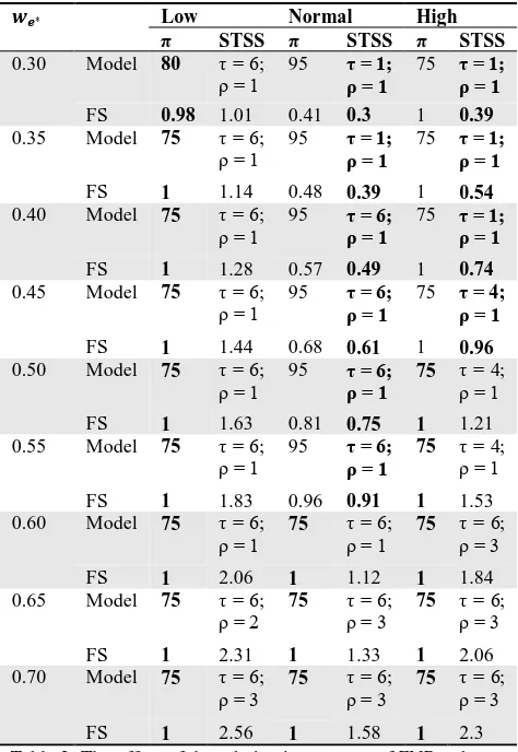
In order to have a better understanding of the effect of detecting high-confidence episodes on the final scores, we have reported the best performing Percentile and STSS based NRC detection models for different ��∗ values ranging from 0.3 to 0.7. The results of this analysis is shown in Table 2. The best performing models and their Final Score (FS) values are highlighted in bold.
��∗ Low Normal High
π STSS π STSS π STSS
0.30 Model 80 τ = 6;
ρ = 1 95 τ = 1; ρ = 1 75 τ = 1; ρ = 1 FS 0.98 1.01 0.41 0.3 1 0.39 0.35 Model 75 τ = 6;
ρ = 1 95 τ = 1; ρ = 1 75 τ = 1; ρ = 1
FS 1 1.14 0.48 0.39 1 0.54
0.40 Model 75 τ = 6;
ρ = 1 95 τ = 6; ρ = 1 75 τ = 1; ρ = 1
FS 1 1.28 0.57 0.49 1 0.74
0.45 Model 75 τ = 6;
ρ = 1 95 τ = 6; ρ = 1 75 τ = ρ = 14;
FS 1 1.44 0.68 0.61 1 0.96
0.50 Model 75 τ = 6;
ρ = 1 95 τ = 6; ρ = 1 75 τ = 4; ρ = 1
FS 1 1.63 0.81 0.75 1 1.21
0.55 Model 75 τ = 6;
ρ = 1 95 τ = 6; ρ = 1 75 τ = 4; ρ = 1
FS 1 1.83 0.96 0.91 1 1.53
0.60 Model 75 τ = 6;
ρ = 1 75 τ = 6; ρ = 1 75 τ = 6; ρ = 3
FS 1 2.06 1 1.12 1 1.84
0.65 Model 75 τ = 6;
ρ = 2 75 τ = 6; ρ = 3 75 τ = 6; ρ = 3
FS 1 2.31 1 1.33 1 2.06
0.70 Model 75 τ = 6;
ρ = 3 75 τ = 6; ρ = 3 75 τ = 6; ρ = 3
FS 1 2.56 1 1.58 1 2.3
Table 2. The effect of the relative importance of FNR values on the best performing NRC models on different travel demand levels
The results add further support to the importance of considering travel demand while developing NRC detection methods. For holidays, due to the low travel demand, the NRCs are much more compact leading to lower LI values. Therefore, the emphasis is on detecting high-confidence episodes; hence, liberal models are preferred. Actually, only when we consider the lowest ��∗ value,
the best performing model is the second most liberal NRC detection model (i.e. π = 80). In the remaining cases the best performing model is indeed the most liberal model. The previous outcome regarding the advantage of liberalising an STSS model by increasing its temporal window size is yet again supported. Only when the ��∗ is increased to 0.65, it became inevitable to further liberalise the method by increasing the spatial window size.
For normal travel demand, it seems that STSS is favoured when the evaluation criteria are weighted equally. However, there is a shift in the preference of both method and model, once the ��∗ is increased from 0.55 to 0.60. In the former case, the most conservative Percentile model is preferred (i.e. π = 95); yet the best performing model is an STSS model (i.e. τ = 6, ρ = 1). Whereas in the latter case the most liberal model (i.e. π = 75) is the best model.
For high travel demand, STSS models show their true advantage for lower values of ��∗. The difference between the FS values are the highest in terms of ratio when ��∗= 0.30. This is because, liberal models perform so poorly with respect to the LI due to their tendency to consider even the slightest increment in LJTs to belong to an NRC. In such high travel demand situations; however, the traffic operation centres might want to localise the spatial sources of congestion in order to develop effective contingency plans. Consequently, conservative models could be favoured in such high demand situations.
5. DISCUSSION AND CONCLUSIONS
The advancement of sensor technology allowed traffic specialists to collect and analyse large amounts of traffic data on a daily basis. Successful applications range from dynamic traffic light control to rapid incident detection to journey time estimation. Accurate detection of NRCs is becoming an emerging research direction within this context, as timely detection of such unexpected events could reduce the overall negative effect.
Previous research efforts on NRC detection have not considered the impact of travel demand on the overall performance of the methods. This paper demonstrated that travel demand has a substantial effect on the performance of the methods. Even though liberal NRC detection models are in favour for low travel demand, this paper demonstrates that increasing travel demand might necessitate favouring the LI criterion in order to pinpoint the source of NRC.
The current research could be extended in several research directions. First is the necessity to develop further evaluation criteria, as the FNR values could be very close to zero in liberal NRC detection models, which may then compromise the calculation of Final Score values. Second, the theory of STSS based NRC detection models could be improved to consider spatial-temporal correlations within the estimated LJTs. Last, further exploration of novel NRC detection models are necessary that would incorporate real-life issues such as missing data.
ACKNOWLEDGEMENTS
This work is part of the STANDARD project – Spatio-Temporal Analysis of Network Data and Road Developments (standard.cege.ucl.ac.uk), supported by the UK Engineering and Physical Sciences Research Council (EP/G023212/1) and Transport for London (TfL). The first author is partially funded through the Research Fund of the Hacettepe University (FDS-2015-8424). The contents of this paper reflect the views of the
Percentile Models π= 75, 80, 85, 90, 95
STSS Models
τ = τ = 2 τ = τ = τ = τ = 6
: Low
: Normal
: High
authors, who are responsible for the facts and the accuracy of the data presented herein. The contents do not necessarily reflect the official views or polices of TfL.
REFERENCES
Anbaroglu, B., Heydecker, B., and Cheng, T. (2014). Spatio-temporal clustering for non-recurrent traffic congestion detection on urban road networks. Transp. Res. Part C Emerg. Technol. 48, 47–65.
Anbaroğlu, B., Cheng, T., and Heydecker, B. (2015). Non-recurrent traffic congestion detection on heterogeneous urban road networks. Transp. Transp. Sci. 11, 754–771.
Arezoumandi, M. (2011). Estimation of Travel Time Reliability for Freeways Using Mean and Standard Deviation of Travel Time. J. Transp. Syst. Eng. Inf. Technol. 11, 74–84.
Beevers, S.D., and Carslaw, D.C. (2005). The impact of congestion charging on vehicle emissions in London. Atmos. Environ. 39, 1–5.
Carrion, C., and Levinson, D. (2012). Value of travel time reliability: A review of current evidence. Transp. Res. Part Policy Pract. 46, 720–741.
Chang, S.-L., Chen, L.-S., Chung, Y.-C., and Chen, S.-W. (2004). Automatic license plate recognition. Intell. Transp. Syst. IEEE Trans. On 5, 42–53.
FHWA (2012). Traffic Congestion and Reliability: Trends and Advanced Strategies for Congestion Mitigation: Executive Summary.
Geroliminis, N., and Sun, J. (2011). Properties of a well-defined macroscopic fundamental diagram for urban traffic. Transp. Res. Part B Methodol. 45, 605–617.
Goodwin, P. (2004). The economic costs of road traffic congestion.
Gronau, R. (1970). The Effect of Traveling Time on the Demand for Passenger Transportation. J. Polit. Econ. 78, 377–394.
Hall, F.L. (2001). Traffic Stream Characteristics. In Traffic Flow Theory: A State-of-the-Art Report, (FHWA/TRB/ORNL),.
Han, L.D., and May, A.D. (1989). Automatic Detection of Traffic Operational Problems on Urban Arterials. Res. Rep. Inst. Transp.
Hollander, Y., and Liu, R. (2008). Estimation of the distribution of travel times by repeated simulation. Transp. Res. Part C Emerg. Technol. 16, 212–231.
Kerner, B.S., and Konhäuser, P. (1994). Structure and parameters of clusters in traffic flow. Phys. Rev. E 50, 54–83.
Kwon, J., Mauch, M., and Varaiya, P. (2006). Components of Congestion: Delay from Incidents, Special Events, Lane Closures, Weather, Potential Ramp Metering Gain, and Excess Demand. Transp. Res. Rec. 1959, 84–91.
Moylan, E., Foti, F., and Skabardonis, A. (2016). Observed and simulated traffic impacts from the 2013 Bay Area Rapid Transit strike. Transp. Plan. Technol. 39, 162–179.
National Research Council (1994). Curbing Gridlock: Peak-Period Fees to Relieve Traffic Congestion -- Special Report 242.
Neill, D.B., and Moore, A.W. (2004). Rapid detection of significant spatial clusters. In Proceedings of the Tenth ACM SIGKDD International Conference on Knowledge Discovery and Data Mining, (New York, NY, USA: ACM), pp. 256–265.
Patil, G.P., and Taillie, C. (2004). Upper level set scan statistic for detecting arbitrarily shaped hotspots. Environ. Ecol. Stat. 11, 183–197.
Polus, A. (1979). A study of travel time and reliability on arterial routes. Transportation 8, 141–151.
Pu, W. (2011). Analytic Relationships Between Travel Time Reliability Measures. Transp. Res. Rec. J. Transp. Res. Board 2254, 122–130.
Robinson, S., and Polak, J. (2006). Overtaking Rule Method for the Cleaning of Matched License-Plate Data. J. Transp. Eng. 132, 609–617.
Schmid, V., and Doerner, K.F. (2010). Ambulance location and relocation problems with time-dependent travel times. Eur. J. Oper. Res. 207, 1293–1303.
Susilawati, S., Taylor, M.A.P., and Somenahalli, S.V.C. (2011). Distributions of travel time variability on urban roads. J. Adv. Transp.
TfL (2010). Travel in London Report 3.
Treiber, M., Hennecke, A., and Helbing, D. (2000). Congested traffic states in empirical observations and microscopic simulations. Phys. Rev. E 62, 1805–1824.
Triantaphyllou, E., and Mann, S.H. (1989). An examination of the effectiveness of multi-dimensional decision-making methods: A decision-making paradox. Decis. Support Syst. 5, 303–312.
Tsapakis, I., Heydecker, B.G., Cheng, T., and Anbaroglu, B. (2013). How tube strikes affect macroscopic and link travel times in London. Transp. Plan. Technol. 36, 109–129.
Wardrop, J. (1952). Some theoretical aspects of road traffic research. Proc. Inst. Civ. Eng. Part II 1.
Yang, H., and Bell, M.G.. (1997). Traffic restraint, road pricing and network equilibrium. Transp. Res. Part B Methodol. 31, 303– 314.