RESEARCH ARTICLE
10.1002/2014MS000317
Impacts of forest harvest on cold season land surface
conditions and land-atmosphere interactions in northern Great
Lakes states
Matthew Garcia1, MutluOzdogan€ 1, and Philip A. Townsend1
1Department of Forest and Wildlife Ecology, University of Wisconsin-Madison, Madison, Wisconsin, USA
Abstract
Land cover change, including temporary disturbances such as forest harvests, can significantly affect established regimes of surface energy balance and moisture exchange, altering flux processes that drive weather and climate. We examined the impacts of forest harvest on winter land-atmosphere interac-tions in a temperate region using high-resolution numerical modeling methods in paired simulainterac-tions. Using the WRF-ARW atmospheric model and the Noah land surface model, we simulated the balance of surface sensible and latent heat fluxes and the development and dissipation of a stable nocturnal boundary layer during generally calm synoptic conditions. Our results show reduced daily-average snow-covered land sur-face sensible heat flux (by 80%) and latent heat flux (by 60%) to the atmosphere in forest clearings due to albedo effects and rebalancing of the surface energy budget. We found a land surface cooling effect (28 W m22) in snow-covered cleared areas, consistent with prior modeling studies and conceptual understanding of the mechanisms for midlatitude deforestation to offset anthropogenic global warming at local scales. Results also demonstrate impacts of forest clearing on the passage of a weak cold front due to altered near-surface winds and boundary layer stability. We show significant differences in both near-surface conditions and fluxes between harvested and undisturbed forest areas. Our results demonstrate the potential utility of high-resolution remote sensing analyses to represent transient land cover changes in model simulations of weather and climate, which are usually undertaken at coarser resolutions and often overlook these changes at the land surface.
1. Introduction
Land cover change can have unanticipated effects on weather [Pielke et al., 2007], climate [Pielke et al., 2002;
Mahmood et al., 2013], hydrology [Chanasyk et al., 2003], carbon dynamics [Goetz et al., 2012], and numerous
other environmental and ecosystem services [Foley et al., 2005]. In particular, forest disturbances may lead to measurable impacts on the energetic and hydrologic balance at the land surface [Kim and Wang, 2007;
Bonan, 2008;Pielke et al., 2011;Anderegg et al., 2012]. Changes in biophysical properties of vegetation and
the underlying soil affect land-atmosphere interactions [Bond, 2000;Barnes and Roy, 2008;Kuusinen et al., 2012], especially the fluxes of energy, moisture, and carbon [Schulze, 1986;Bonan, 2008;Katul et al., 2012]. Both observations and modeling studies indicate that the removal of forest from the landscape has particu-lar impacts on the interaction of various components in the land-atmosphere system [Strassmann et al., 2008;Pielke et al., 2011]. Such changes are evident in cycles of vegetation phenology and can influence lon-ger term trends in vegetation health and growth [Bond, 2000]. Satellite-based remote sensing has broad utility for the mapping of vegetation state and disturbance at moderate and high resolution (on the order of 10 m–1 km spatial scales) over large areas and long times [Xie et al., 2008;Frolking et al., 2009]. Using remote sensing products and detailed numerical modeling methods, we explore the extent to which indus-trial forest harvest practices—defined as partial and clear-cut removal of trees for commercial purposes without permanent land use change—may modify weather-related and hydrologic processes in and near intensely managed locations.
In the middle and high latitudes, researchers have found a cooling effect on the climate system due to the albedo-related impacts of forest clearing [Gibbard et al., 2005]. As well, the carbon-cycle impacts of defores-tation can further complicate our understanding of the effects of forest clearing in the climate system [Bala
et al., 2007;Bala and Nag, 2012]. At present, the effects of forest clearing on weather and climate can be
Key Points:
Land cover change alters land-atmosphere energy and moisture exchange
Forest clearing significantly reduces winter sensible and latent heat fluxes
High-resolution land cover change analyses may be useful in synoptic models harvest on cold season land surface conditions and land-atmosphere
Accepted article online 26 AUG 2014
This is an open access article under the terms of the Creative Commons Attribution-NonCommercial-NoDerivs License, which permits use and distribution in any medium, provided the original work is properly cited, the use is non-commercial and no modifications or adaptations are made.
seen as a collection of fine-scale anthropogenic impacts. With broad-scale land cover and land use change, these accumulating effects may have a more significant impact on broad-scale conditions. Models offer an approach to build our understanding of how local impacts of forest clearing influence parameterizations in and outcomes of coarse-resolution climate models. Such an effort may be compared with recent efforts at cloud-oriented ‘‘superparameterizations’’ [Khairoutdinov and Randall, 2001;Randall et al., 2003] and ‘‘multi-scale modeling frameworks’’ [Tao et al., 2009]. In this paper, however, we concentrate on local rather than global consequences of forest clearing.
Surface albedo, mechanical roughness, and soil moisture are key land surface variables that affect land-atmosphere fluxes at the local scale and thus exert significant influence on atmospheric boundary layer (BL) character and behavior [Garratt, 1993;Sun and Bosilovich, 1996;Santanello et al., 2005]. Heat and moisture exchanges between the surface and free atmosphere shape the stability of the BL and determine the rela-tive ease with which fluxes through the BL occur [Troen and Mahrt, 1986]. The stability of the BL can affect the passage of shallow cold fronts [Smith and Reeder, 1988], further complicating the impacts of surface dis-turbances on local weather conditions. With demonstrated differences in surface conditions and land-atmosphere fluxes between harvested and intact forests, it becomes important to consider spatiotemporal variation of specific vegetation characteristics for the accurate representation of the land surface in coupled modeling systems for meteorology and climate. Model spatial resolution remains an important considera-tion with regard to the dynamic capabilities of BL parameterizaconsidera-tions at 100 m–1 km scales [Horvath et al., 2012], the ‘‘terra incognita’’ [Wyngaard, 2004] at which BL turbulence may be explicitly resolved in the model, especially under convectively unstable conditions [Zhou et al., 2014]. However, these are also the scales at which land cover change is often observed. Most global models are applied at spatial resolutions too coarse to capture the details of these land cover changes and are not formulated to account for the physical mechanisms of change processes [Dirmeyer et al., 2006]. Careful application of a scale-spanning modeling system to address both high-resolution land characterization and large-scale atmospheric dynam-ics may provide a better understanding of the local (but widely accumulating) land cover change impacts on weather and climate.
2. Methods
2.1. Model Description and Forcing Data
We employ version 3.4 of the nonhydrostatic, primitive equation Weather Research and Forecasting (WRF) model with the Advanced Research WRF (ARW) dynamical core physics package [LeMone et al., 2010a, 2010b;Trier et al., 2011]. Atmospheric optical physics are handled by the Goddard radiative parameteriza-tions in both shortwave [Chou, 1990, 1992] and longwave [Chou and Suarez, 1994] spectral ranges. The Grell-Devenyi ensemble cumulus parameterization scheme [Grell and Devenyi, 2002] is employed along with the WRF single-moment five-class (WSM5) microphysics scheme [Hong et al., 2004], although no cumulus convection and only a trace of snowfall (coincident with, and likely forced by, a weak frontal passage as described below) is observed in the study area during our simulated winter conditions. We employed the Yonsei University (YSU) boundary layer (BL) scheme [Hong et al., 2006] with an improved treatment of verti-cal mixing [Hu et al., 2013] and an associated surface layer treatment based on the PSU MM5 modeling sys-tem [Grell et al., 1994]. These selections use BL similarity theory formulations developed for several stability regimes [Zhang and Anthes, 1982] and rely on the surface friction velocityu*that is tied directly to the land cover representation. A convectively stable boundary layer is present at all times during the simulations in this work and mitigates much of the uncertainty related to application of these BL and surface layer schemes at high spatial resolution [Horvath et al., 2012], which can be troublesome in convectively unstable conditions with strong mixing [Zilitinkevich et al., 2008;Zhou et al., 2014].
The WRF-ARW modeling system includes the unified version of the community Noah land surface model (LSM) [Pan and Mahrt, 1987;LeMone et al., 2008]. The community Noah LSM is classified as a second-generation land surface parameterization [Sellers et al., 1997] that simultaneously solves the energy and water balance at the atmosphere-vegetation-soil (or -snow) interface using the corresponding flux-oriented parameters for each of these layers. We employ LSM parameter values that are available in the standard Noah LSM look-up tables included in the WRF-Noah package. Although the Noah LSM remains an attractive choice for its usage across both academic and operational modeling efforts [Ek et al., 2003], the WRF-ARW
Journal of Advances in Modeling Earth Systems
10.1002/2014MS000317
modeling system also now includes the Noah Multi-Physics (MP) LSM [Niu et al., 2011;Yang et al., 2011]. Noah MP is consid-ered a third-generation land surface param-eterization that adds several carbon accounting pools and processes to the Noah LSM and may be employed in our ongoing work as mentioned above.
For the snow cover that persists through our simulation period, the Noah LSM employs a bulk snow representation [Slater
et al., 2001] where a single layer of snow
occupies patches within a grid cell up to a specified limit of snow depth, above which the snow covers the entire grid cell at the same depth. The handling of the soil column temperature and moisture profile accounts for frozen ground conditions [Koren et al., 1999], affecting heat transfer between soil and snow layers and the capability for infiltration of snowmelt and runoff at near-freezing conditions. Some persistent biases previously observed in Noah LSM simulations, such as excessive rates of sublimation and a tendency for early spring snowmelt in mountain regions, have been addressed with several revisions to the snow physics [Livneh et al., 2010;Wang et al., 2010] including the introduction of a time-dependent approxima-tion of snow albedo that diminishes with the age of the snow cover [Barlage et al., 2010].
Our simulation domain is defined by five nested grid layers in a telescoping configuration (Table 1 and Figure 1). The outermost (coarsest) grid, not shown in Figure 1 due to its large spatial coverage, is cen-tered on 45.6N, 91.2W and has a cell size of 30 km to approximate that of the applied meteorological forcing data set. Grid span and cell sizes (and the simulation time step) are reduced progressively to the innermost (finest) grid at ratios that conform to the general advice given in WRF-ARW documentation. The finest grid, listed as ‘‘Grid 5’’ in Table 1, covers an area 20320 km surrounding the study location
at 46.42N, 91.52W at 100 m resolution. The spatial resolutions of Grids 4 and 5 are selected to provide an adequate representa-tion of forest harvest activities at the land surface, considering both the native resolution of Landsat images used for analysis of those activities (30 m) and a character-istic size of forest ownership plots in many areas of the United States. Specifically, a forest parcel that covers 16.2 ha (40 acres) would occupy about 180 Landsat pixels in the land cover change analysis, providing a detailed view of the extent and severity of the harvest activity. However, this translates to only 16 cells in Grid 5 and only a single grid cell on Grid 4. We strike a balance here between the apparent small-scale capabilities of the BL and surface layer parameterizations [Horvath
et al., 2012;Hu et al., 2013], the
availability of high-resolution land cover information from Landsat,
Table 1.General Characteristics of WRF-ARW Model Grids Specified for Our Simulationsa
Grid No. Span (km) Spatial Resolution Source of Land Cover Map 1 2910 30 km 2006 NLCD, aggregated
to required resolution using dominant land cover category 2 570 6 km
3 114 1.2 km
4 38.4 400 m Landsat analysis, aggregated to required resolution 5 20 100 m Landsat analysis; see Figure 2
and text description
aGeographic locations of Grids 2–5 are shown in Figure 1; land cover
for Grid 5 is shown in Figure 2.
adequate representation of forest harvest areas at a land parcel size characteristic to the region, and model developers’ guidance regard-ing telescoped grid configurations in the simulation domain [Skamarock
et al., 2008].
Synoptic atmospheric and surface forc-ing conditions for our simulations were derived from the North American Regional Reanalysis (NARR) data set
[Mesinger et al., 2006;Luo et al., 2007]
at 3 h intervals and a spatial resolution of 0.33(32 km). Our simulation grids
employ the same vertical configuration of atmosphere and soil layers provided in the NARR input. The WRF Prepro-cessing System (WPS) was employed for interpolation from the NARR grid to the 30 km resolution of our outermost simulation grid and to establish initial conditions in the four internal (nested) grids. Following the initial time, NARR forcing conditions are applied only to the outermost (coarsest) simulation grid (‘‘Grid 1’’ in Table 1); synoptic-scale meteorological forcing is thus propa-gated to the internal grids only through the model physics and the numerical formulation of grid nesting. Conditions on the internal grids at mesoscale and convective scale then evolve from established initial condi-tions in dynamical connection with large-scale atmospheric patterns and disturbances and are allowed to feed back to the continued evolution of the model atmosphere and surface conditions.
2.2. Experimental Design
Our study area is located in northwestern Wisconsin (Figure 1) on a glacial outwash plain characterized mostly by jack pine (Pinus banksiana) forests interspersed with stands of red pine (Pinus resinosa), white pine (Pinus strobus), and northern hardwood species. Dense commercial forest parcels often appear in aerial and satellite images as polygonal blocks where clear-cut rotation harvests occur. A map of forest harvest areas for our simulation domain was derived using 30 m Landsat images (WRS-2 Path 26, Row 28) at 5 year intervals for 1985–2010 following the forest change detection method developed byOzdogan€ [2014]. Briefly,Ozdogan employed pair-wise comparisons of Kauth-Thomas tasseled cap transforms [€ Crist and
Cicone, 1984;Crist and Kauth, 1986;Collins and Woodcock, 1996] within a support vector machine (SVM)
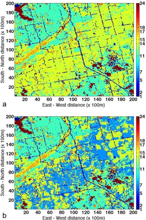
framework [Huang et al., 2002;Mountrakis et al., 2011] to classify harvested areas. To generate a complete land cover map at high spatial resolution for our simulations, the Landsat-based forest harvest maps were then merged with the 2006 USGS National Land Cover Database (NLCD) [Fry et al., 2011]. In this work, we consider two land cover scenarios (Figure 2): for the ‘‘experiment,’’ pixels identified as harvested in the change map were classified with the NLCD Grassland/Herbaceous category; for the ‘‘control,’’ all of these pixels were reclassified as Evergreen Forest. Standard Noah LSM parameter values, as well as spatial coverage within the finest simulation grid, for each of the land cover types shown in Figure 2 are listed in Table 2. Note that the land cover map used for the experiment scenario does not correspond to anyspecific Figure 2.Land cover classifications for Grid 5, covering 20320 km at 100 m
spa-tial resolution, for (a) control and (b) experiment scenarios. Classification index val-ues are noted at right and referenced to the land cover categories listed in Table 2.
Journal of Advances in Modeling Earth Systems
10.1002/2014MS000317
land cover configuration in our study area during 1985–2010, but instead to theaccumulatedharvest activ-ity that was observed in our study area over that period.
Case study dates were selected using National Climatic Data Center (NCDC) daily records of climatological observations at two locations near the study site, shown in Figure 1: Eau Clair Regional Airport (marker ‘‘E’’ in Figure 1; GHCND USW00014991) and Solon Springs (marker ‘‘S’’ in Figure 1; GHCND USC00477892). The period 17–20 February 2001 was identified as an ideal winter case, with 25 cm or more snow on the ground and all daytime temperatures remaining below 0C over that period at both locations. Our focus was
ini-tially on relatively calm days in this period for an examination of winter our study area on 19 Feb-ruary 2001, providing an
Table 2.Land Cover Categories and Standard Noah LSM Parameter Values in the Control (Forested) and Experiment (Harvested) Scenarios for the Maps Shown in Figure 2 Land Cover Category Noah LSM Parameters
Spatial Coverage 1 Urban and builtup land 0.15 0.46 0.880 1.00 200 0.50 7.17 2 Dryland cropland/pasture 0.17–0.23 0.66 0.92–0.985 1.56–5.68 40 0.05–0.15 0.20 5 Cropland/grassland mosaic 0.18–0.23 0.68 0.92–0.98 2.29–4.29 40 0.05–0.14 0.17 7 Grassland 0.19–0.23 0.70 0.92–0.96 0.52–2.90 40 0.10–0.12 0.00 26.54 11 Deciduous broadleaf forest 0.16–0.17 0.58 0.93 1.85–3.31 100 0.50 32.95 30.73 14 Evergreen needleleaf forest 0.12 0.52 0.95 5.00–6.40 125 0.50 41.57 17.23 15 Mixed forest 0.17–0.25 0.53 0.93–0.97 2.80–5.50 125 0.20–0.50 10.59 17 Herbaceous wetland 0.14 0.68 0.95 1.50–5.65 40 0.20 0.33 18 Wooded wetland 0.14 0.50 0.95 2.00–5.80 100 0.40 3.31 24 Snow or ice 0.55–0.70 0.82 0.95 0.01 0.001 3.72
Table 3.Differences in Aggregated Values of Selected Variables Between Experiment and Control Scenariosa
Variable (Model Name) (Units)
Harvest Areas in Grid 5 Stable Forest or Other Land Cover in Grid 5 Full Grid 5
All Intervals Daytime Nighttime All Intervals Daytime Nighttime All Intervals Daytime Nighttime
l r l r l r l r l r l r l r l r l r
Temperature at 2 m (T2) (K)
20.58 0.53 20.24 0.24 20.83* 0.55 0.02 0.03 20.06 0.07 0.02 0.03 20.16 0.12 20.11 0.08 20.20 0.13
Humidity at 2 m (Q2) (kg/kg)
28.46E-6 1.33E-5 21.99E-5 1.29E-5 2.68E-7 3.17E-6 22.37E-6 5.35E-625.85E-6 6.59E-6 2.84E-7 9.94E-7 23.99E-6 7.02E-6 29.58E-6 7.48E-6 2.79E-7 1.47E-6
Wind speed at 10 m (calculated) (m/s)
0.42*** 0.32*** 0.61*** 0.22** 0.28*** 0.31*** 0.13* 0.03 0.13 0.04 0.14* 0.03 0.21*** 0.10* 0.26** 0.07 0.17** 0.10*
Sensible heat
flux (SH) (W/m2) 2
13.5*** 23.6*** 234.8*** 21.7*** 2.79*** 3.31 20.11 0.86 0.57 0.85 20.63 0.36 23.66 5.75** 28.82* 5.36 0.28 0.72
Latent heat
flux (LH) (W/m2) 2
7.58*** 9.29*** 216.0*** 8.58*** 21.18*** 1.21* 0.01 0.29 0.12 0.37 20.07 0.16 22.00 2.39** 24.15* 2.21 20.37 0.32
Ground heat flux
(GRDFLX) (W/m2) 2
0.19 6.43*** 3.94* 5.70*** 23.34 5.02** 20.01 0.54 0.44 0.49 20.35 0.22 20.06 1.94 1.37 1.69 21.15 1.31
Moisture flux
(QFX) (kg/m2/s) 2
2.66E-6*** 3.77E-6***26.06E-6*** 3.50E-6***26.80E-8** 3.30E-7*** 2.32E-8 9.26E-8 4.54E-8 1.34E-7 6.15E-9 2.58E-8 26.90E-7 9.80E-7*** 21.58E-6** 9.10E-7* 21.35E-8 7.30E-8***
Stability (calculated) (K m/s)
9.74E-4 1.29E-3* 7.09E-4 1.32E-3 1.18E-3 1.22E-3 2.29E-4 4.42E-4 2.07E-4 5.35E-4 2.46E-4 3.55E-4 4.27E-4 5.32E-4 3.40E-4 5.09E-4 4.93E-4 5.41E-4
aAsterisks indicate differences between the control and experiment simulations at significance levels of *p<0.05, **p<0.01, or ***p<0.001 by Student’sttest (for mean values) orFtest (for variance). The notation
‘‘E-N’’ indicates ‘‘3102N.’’ Land-atmosphere fluxes are generally signed with positive values for upward fluxes, i.e., from the land surface to the atmosphere, but the ground heat flux is signed in the opposite manner, with positive values indicating heat transfer from the model soil layers to the deep soil column. Stability is calculated in the 1000–900 hPa layer from model output fields during postprocessing (see Appendix A).
Journal
o
f
A
dvances
in
M
odeling
E
arth
Systems
1
0
.1
002/20
14MS000
317
GARCIA
ET
AL.
VC
2014.
The
Authors.
front through the simula-tion domain.
Simulations were exe-cuted on a parallel super-computing system and were undertaken as a pair to examine the differen-ces between control (‘‘for-est’’) and experiment (‘‘harvest’’) conditions on Grid 5. Inputs to the two scenarios in the simulation pair therefore differ only in their land cover maps applied at the two finest modeling grids with 100 m (Grid 5) and 400 m (Grid 4) resolutions. Land cover on the coarser model grids (Grids 1–3) did not differ across the simulation pair and was determined by resampling and aggregation using the default USGS land cover map with a base spatial resolution of 30 arc sec (1 km), which is pro-vided with the WPS pack-age and is consistent with the NARR forcing data set. Of our 4 day simulation period 17–20 February 2001, we used the first day as a model spin-up period, and results from only the subsequent simulation days are analyzed.
3. Results
Results from the experiment and control scenarios were generated for Grid 5 at 5 min intervals during the 4 day simulation period, with the 3 days after the first ‘‘spin-up’’ day compared as follows. First, a binary mask was calculated using the two land cover maps in Figure 2 to isolate those areas of Grid 5 that changed between scenarios (entirely forest/grassland areas) and those areas that remained consistent across the experiment (lakes, roads, and some forest areas). Then, time series of the several output varia-bles of interest were spatially aggregated using the binary mask at each time over (a) the area subjected to forest harvest within Grid 5, (b) the area of stable forest or other land cover within Grid 5, and (c) across all of Grid 5 (Table 3, main column divisions). These calculations produced time series of mean and var-iance of model output variables for each spatial area of aggregation. We compared (a) all times, (b) day-time, and (c) nighttime periods (Table 3, subcolumns) to isolate any day/night differences and to detect indicators of nocturnal boundary layer development, especially in the harvested areas. We used a two-tailed Student’sttest andFtest to determine statistical significance of the differences between one-dimensional time series of scenario results at these nine spatiotemporal resolutions. Asterisks in Table 3 indicate the level of test significance. In addition, the time series for each spatial and temporal aggrega-tion were differenced (diff5experiment-control) and the mean and variance of that difference time series is listed in the cells of Table 3. Note that these aggregated and summarized values in Table 3 cover the 3 day evaluation period of the simulation and are not explicitly segregated to account for changing dynamical conditions within that time, such as the cold front passage.
3.1. Surface Temperature and Wind Speed
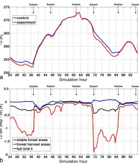
The nighttime reduction of sur-face temperature in the experi-ment scenario that is shown in Figure 3 is statistically significant (p<0.05). The greater
near-surface mean wind speed in for-est harvfor-est areas for the experi-ment scenario is also statistically significant (p<0.001) in all
tem-poral aggregations and leads to some significant differences when averaged over the entire finest grid as well (p<0.01).
Time series of the surface wind speed in the area of forest har-vest are shown in Figure 4a, and differences between the two scenarios over the three areas of spatial aggregation are shown in Figure 4b. At all levels of spatial and temporal aggregation, the near-surface wind speed mean and variance increased in the experiment (harvest) scenario.
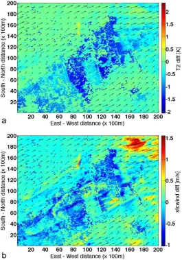
The largest differences in surface temperature between control and experiment scenarios occur at night, especially during calm periods with near-surface wind speeds generally less than 4 m s21
. These can be related to the establishment of a cold noctur-nal boundary layer that is appa-rent in cleared areas. Harvest areas are2 K colder than surrounding forest areas just prior to sunrise on 18 February (Figure 5a) and generally have near-surface wind speeds1 m s21
less than surrounding areas at the same time (Figure 5b). Similar condi-tions are found just prior to sunrise on 20 February as well. Animated simulation results indicate on both of these mornings that greater daytime wind speeds propagate downward from the free atmosphere (above900 hPa) and erode the stable nocturnal boundary layer within 20–30 min after sunrise. This is evident in the far northeast-ern portion of Figure 5, where surface warming and near-surface wind speeds begin to increase at the time of that snapshot. Differences in near-surface wind speeds between the control and experiment scenarios are gener-ally larger during daytime hours and through the period of frontal disturbance on 19 February.
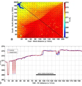
We identified the time of frontal passage over Grid 5 in our simulation domain as approximately 1515 UTC (0915 LST) on 19 February 2001. This is a relatively weak cold front, with an immediate postfrontal tempera-ture depression of 1 K, but with temperatempera-ture reductions as much as 3K in the farther postfrontal region (Figure 6a). The passage of the cold front appears to eliminate any differences in surface temperature between the control and experiment scenarios, both over the harvest areas and over forest and lake areas several minutes later. The passage of the front over Grid 5 is accompanied by a trace snowfall event, due to relatively moist surface air forced over the advancing frontal boundary.
The position of the front is indicated by the sharp temperature gradient in both cross section (Figure 6b) and map representations. At 1445 UTC, the fronts in each scenario show a position difference of only a few
Figure 5.Mapped differences between experiment and control scenarios of (a) surface tem-perature and (b) near-surface wind speed at 1330 UTC (0730 LST) on 18 February 2001, showing variations in modeled conditions just prior to sunrise. Similar conditions are simu-lated around the same time on 20 February as well.
Journal of Advances in Modeling Earth Systems
10.1002/2014MS000317
hundred meters, but this difference increases to nearly 500 m by 1505 UTC, just prior to pas-sage of the cold front over the largest area of forest harvest in the experiment scenario (see Figure 2b). While the cold front then contin-ues over an unbroken forest area in the control scenario, the front in the experiment scenario speeds up, and their positions are nearly identical at 1525 UTC just before exiting the harvest region. The cross-frontal tempera-ture gradient in the experiment scenario is also weakened by that time to less than 1 K over a slightly wider zone. By 1545 UTC, the front in the experiment scenario passes again over rougher forest areas in the southeastern portion of Grid 5, where the cross-frontal temperature gradi-ent is again strengthened but its progress is slowed, and the position difference between scenarios again increases to nearly 500 m.
3.2. Surface Fluxes and Energy Balance
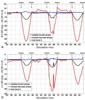
Land-atmosphere fluxes also show the greatest differences between control and experiment scenarios dur-ing the daytime, with local energetic balance drivdur-ing the surface fluxes through those hours. Insolation reaches peak daytime values of650 W m22, and the surface albedo of the forest and harvested areas (Table 1) accounts for much of the difference in energetic balance between scenarios. Within forest harvest areas, the sensible heat (SH) flux in the experiment scenario is reduced by65 W m22from the control sce-nario during the day (Figure 7a), although smaller differences are found during the period of frontal passage on 19 February. The experimental daytime latent heat (LH) flux is likewise reduced from the control scenario by 25 W m22(Figure 7b), with larger differences during the date of frontal passage. Warmer temperatures on that day lead to a slight melting of the existing snow cover in Grid 5. On the less disturbed days of the simulation period, the midday peak in SH flux is apparent in Figure 8 where the pattern of forest harvest areas is clearly visible. The spatial pattern of the peak (midday) LH flux is the same, although its magnitude in the cleared areas is smaller.
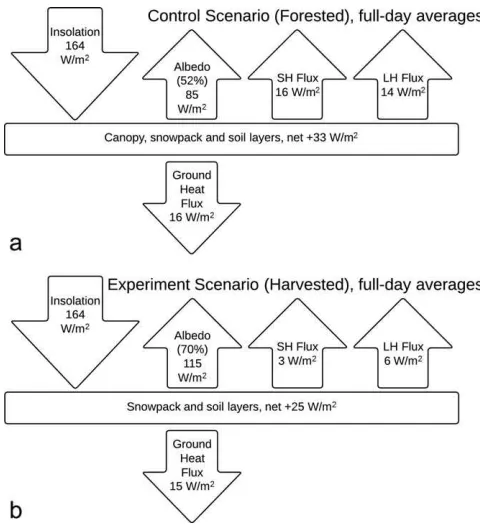
Figure 9 summarizes the modeled land surface energy balance for the areas in Grid 5 of our simulation domain that were subjected to forest harvest. In these diagrams, fluxes (arrows) were calculated from model simulation results as the average of that flux component over the 3 day period (including nights) and the residual of that calculation is assigned as the net land surface heat flux. The differences between control (forested, Figure 9a) and experiment (harvested, Figure 9b) scenarios are driven primarily by the large differ-ence in surface albedo and the partitioning of remaining energetic fluxes to sensible and latent heating.
The Bowen ratio, defined as the ratio of sensible to latent heat exchange orB5SH/LH, actually shifts between these two scenarios. In forested conditions (Figure 9a),B51.14 suggests that the surface energy balance is affected almost equally by the temperature difference between land and atmosphere (driving SH
exchange) and by the use of energy in the snow-pack for melting, evapo-ration, and sublimation, and in the forest for tran-spiration processes (the paths of LH exchange). In the harvest scenario (Fig-ure 9b), values of SH and LH are both smaller than in nonlogged conditions (attributable in large part to the albedo difference between scenarios), but
B50.5 suggests a strong shift toward greater energy allocation to melt-ing, evaporation, and sublimation processes in the exposed snowpack. The exposed snow sur-face in forest harvest areas effectively insulates the soil surface, which retains less of the insola-tion heat flux than the forested areas in the con-trol scenario. Overall, our simulations suggest that forest clear-cutting is equivalent to a net local land surface heat flux of
28 W m22under winter, snow-covered conditions.
4. Discussion and
Conclusions
The most significant changes in surface states, flux variables, and bound-ary layer processes between intact and har-vested forests resulted from the differences between input land cover maps and their represen-tation by the LSM param-eterization. For example, departures in tempera-ture were tied most gen-erally to the differences in albedo, emissivity, and snow depth between
Figure 7.Time series for the differences between control and experiment scenarios of surface (a) sensible heat (SH) flux and (b) latent heat (LH) flux as aggregated over stable forest areas in Grid 5, harvested areas in Grid 5, and averaged over all of Grid 5.
Figure 8.Mapped differences between experiment and control scenarios of surface sensible heat (SH) flux at 1800 UTC (1200 LST) on 18 February 2001, showing the variation between forested and cleared areas in Grid 5 near the midday peak of surface heat fluxes. A map of latent heat (LH) fluxes (not shown) is qualitatively similar in pattern, but of smaller magnitude in the cleared areas.
Journal of Advances in Modeling Earth Systems
10.1002/2014MS000317
control (forested) and experiment (harvested) land covers, as well as the role of these conditions within the model in the energetic balance at the land surface. Differences in wind speed can be attributed to the diminished roughness of grass and snow surfaces compared to the forest canopy in the control scenario. Simulated latent heat fluxes were greater on 19 February than on previous or subsequent days, which can be attributed to higher surface temperatures around the time of frontal passage and a greater partition of available energy to melting and evaporation in the snow cover of exposed clear-ings. The strength of the front, characterized most simply as the cross-frontal temperature gradient, remained steady over time in the control scenario but was weakened in the experiment upon passage over the harvested area. While fron-tal dynamics can be complex over heterogeneous surfaces, we attribute these differences primarily to the obvious variations in surface rough-ness between the forest and harvested (grassland/snow) cover types, as well as to the collection of colder, more stable air near the surface in the harvested areas prior to frontal passage (Table 3).
Although the surface energy balance can be evaluated at an individual point within this model, where a vegetation/soil column in the LSM does not communicate with its neighbors, wind-based atmospheric transfer of energy and momentum between locations can still alter the atmospheric kinematic and thermo-dynamic balance in the surrounding area. Harvest-induced changes in surface temperature, humidity, and wind speed in disturbed areas are thus tied dynamically to the surrounding intact forest. This points to the need to evaluate impacts of land cover disturbance at scales larger than the individual forest clearing, at which both the occurrence and pattern of disturbances become important. Future work will examine larger areas of forest change, may involve more detailed analyses of changes in atmospheric (e.g., frontal) dynam-ics due to differences in surface roughness and sensible heat fluxes, and will address hydrological (e.g., run-off and soil moisture) impacts of disturbances to vegetation. In a manner similar to this work, we plan to evaluate surface energetic and hydrologic balance changes due to forest disturbances of several types and severities, under several meteorological scenarios including winter snow cover and both winter and summer snow-free conditions. In this work, we have specifically addressed the local energy and moisture balance, but not the carbon cycle, at the land surface. Our approach can be extended with alternative mod-els that consider more completely the role of forest harvest in the intertwined energy, moisture, and carbon cycles of the global climate system.
This study was conducted on the premise that high-resolution (30–100 m pixel scale) remote sensing obser-vations of forests [Xie et al., 2008;Ozdogan€ , 2014] provide useful information to quantify the impacts of local and regional disturbances on the land-atmosphere energy balance [Bonan et al., 2002;Sterling and
Ducharne, 2008]. The results are consistent with a conceptual understanding of the impacts of forest harvest
on the climate system in middle and high latitudes, specifically the cooling effect of exposed snow surfaces in winter [Snyder et al., 2004;Bonan, 2008]. Our high-resolution experimental results at the local scale are also consistent with large-scale simulations of deforestation impacts obtained using coarser modeling grids
[Snyder et al., 2004;Gibbard et al., 2005;Bala et al., 2007;Klingaman et al., 2008;Mishra et al., 2010]. In
extending such modeling capability to landscape-scale and stand-scale forest dynamics, we provide further
support for the use of remote sensing-based land cover change data in numerical analysis of
land-atmosphere fluxes and energetic balance. In particular, we demonstrate the relevance of such efforts in forest regions subject to natural and anthropogenic disturbances, even where the changes are transient in time and discontinuous in space. High spatial resolution land cover data derived from remote sensing imagery (e.g., Landsat) provide context to quantify the potential impacts of harvest and other disturbances and their feed-backs to the meteorology and microclimate at local and downwind/downstream locations [Pielke and Avissar, 1990]. We have demonstrated relevant impacts on evapotranspiration processes that may be important to hydrologic balance in disturbed forests [Sun et al., 2008] and, along with local temperature changes, may influ-ence the survivability of regenerating forests after disturbance [Groot and King, 1993;Pauli et al., 2013]. While we have focused on a single-case modeling approach, an ensemble implementation could illustrate the differ-ent sensitivities of model results to variations in boundary and surface layer formulations, parameter input val-ues, and atmospheric forcing conditions. Many aspects of BL dynamics in land-atmosphere model
formulations remain limited by the model vertical resolution, traditional BL parameterizations, and overlooked impacts of the forest canopy as a semipermeable surface layer [Ross, 2012]. The model BL formulation is sensi-tive to spatial resolution in the representation of turbulence near the land surface. However, we expect that calm and stable BL conditions with weak mixing at low Richardson numbers (the ratio of buoyant to shear forces) [Zilitinkevich et al., 2008] could mitigate some of the grid-scale sensitivity [Wyngaard, 2004;Horvath
et al., 2012] that is more often linked to a convectively unstable BL [Zhou et al., 2014], with greater turbulence
and strong mixing at large Richardson numbers. We have used a high-resolution numerical modeling system, with close ties to operational numerical weather prediction models, to demonstrate some important effects of forest harvest that are not typically accounted at the grid scale in larger (continental) domains and may be overlooked in subgrid parameterizations applied to global modeling efforts. Our results (Table 3) show that several relevant, flux-related model variables achieve significant departures from control conditions over the course of an experimental scenario in which less than 30% of the land cover within the grid domain was changed. Likewise, the energy balance at the land surface was altered to a degree that exceeds anthropo-genic forcing due to modeled emission scenarios that are reported in the climate change literature [e.g.,IPCC, 2013], with the potential to offset global forcing at local scales.
Appendix A: Calculating Boundary Layer Stability
The near-surface stability is calculated using model output fields in the lowest five levels of the atmospheric column, between 1000 and 900 hPa (at 25 hPa intervals), for which the vertical velocitywis available. The 1000 hPa level is very close to the actual ground surface in the model formulation, and the 900 hPa level occurs above the atmospheric BL in the simulations examined here. The BL stability is defined afterStull
[1988, p. 171] as
stability52w0
h0m (A1)
where the virtual potential temperature is calculated as
hm5hð110:608qÞ (A2)
and the values ofh(potential temperature) andq(water vapor mixing ratio) are given in model output at the required atmospheric levels. We have elected to reverse the sign of the calculated value in order to bet-ter associate positive values with BLstabilityand negative values with BLinstability. Reynolds averaging is used here only in the vertical dimension as
w5 1
NðkÞ
X900 hPa
k51000 hPawk forNðkÞ55 (A3)
to obtain the vertical mean and
wk05wk2w fork51000 hPa…900 hPa at 25 hPa intervals (A4) to obtain the perturbation from the vertical mean at each level. Similar calculations are performed forhv
and the product of the two perturbations. Spatial aggregation over the areas listed in Table 3 (‘‘harvest areas,’’ other areas, and ‘‘full Grid 5’’) then fulfills Stull’s instruction that the BL stability should be evaluated on a ‘‘nonlocal’’ (i.e., not on an individual grid point) basis.
Journal of Advances in Modeling Earth Systems
10.1002/2014MS000317
References
Anderegg, W. R. L., J. M. Kane, and L. D. L. Anderegg (2012), Consequences of widespread tree mortality triggered by drought and temper-ature stress,Nat. Clim. Change,3, 30–36, doi:10.1038/nclimate1635.
Bala, G., and B. Nag (2012), Albedo enhancement over land to counteract global warming: Impacts on hydrological cycle,Clim. Dyn.,39, 1527–1542, doi:10.1007/s00382-011-1256-1.
Bala, G., K. Caldeira, M. Wickett, T. J. Phillips, D. B. Lobell, C. Delire, and A. Mirin (2007), Combined climate and carbon-cycle effects of large-scale deforestation,Proc. Natl. Acad. Sci. U. S. A.,104, 6550–6555, doi:10.1073/pnas.0608998104.
Barlage, M., F. Chen, M. Tewari, K. Ikeda, D. Gochis, J. Dudhia, R. Rasmussen, B. Livneh, M. Ek, and K. Mitchell (2010), Noah land surface model modifications to improve snowpack prediction in the Colorado Rocky Mountains,J. Geophys. Res.,115, D22101, doi:10.1029/ 2009JD013470.
Barnes, C. A., and D. P. Roy (2008), Radiative forcing over the conterminous United States due to contemporary land cover land use albedo change,Geophys. Res. Lett.,35, L09706, doi:10.1029/2008GL033567.
Bonan, G. B. (2008), Forests and climate change: Forcings, feedbacks, and the climate benefits of forests,Science,320, 1444–1449, doi: 10.1126/science.1155121.
Bonan, G. B., S. Levis, L. Kergoat, and K. W. Oleson (2002), Landscapes as patches of plant functional types: An integrating concept for cli-mate and ecosystem models,Global Biogeochem. Cycles,16(2), 1021, doi:10.1029/2000GB001360.
Bond, B. J. (2000), Age-related changes in photosynthesis of woody plants,Trends Plant Sci.,5, 349–353, doi:10.1016/S1360-1385(00)01691-5.
Chanasyk, D. S., I. R. Whitson, E. Mapfumo, J. M. Burke, and E. E. Prepas (2003), The impacts of forest harvest and wildfire on soils and hydrology in temperate forests: A baseline to develop hypotheses for the Boreal Plain,J. Environ. Eng. Sci.,2, S51–S62, doi:10.1139/s03-034.
Chou, M.-D. (1990), Parameterization for the absorption of solar radiation by O2and CO2with application to climate studies,J. Clim.,3,
209–217, doi:10.1175/1520-0442(1990)003<0209:PFTAOS>2.0.CO;2.
Chou, M.-D. (1992), A solar radiation model for climate studies,J. Atmos. Sci.,49, 762–772, doi:10.1175/1520-0469(1992)049< 0762:ASRM-FU>2.0.CO;2.
Chou, M.-D., and M. J. Suarez (1994), An efficient thermal infrared radiation parameterization for use in general circulation models,
Technical Report Series on Global Modeling and Data Assimilation, Tech. Memo. 104606, vol. 3, 102 pp., Goddard Space Flight Center, Greenbelt, Md.
Collins, J. B., and C. E. Woodcock (1996), An assessment of several linear change detection techniques for mapping forest mortality using multitemporal Landsat TM data,Remote Sens. Environ.,56, 66–77, doi:10.1016/0034-4257(95)00233-2.
Crist, E. P., and R. C. Cicone (1984), A physically-based transformation of Thematic Mapper data: The TM Tasseled Cap,IEEE Trans. Geosci. Remote Sens.,22, 256–263, doi:10.1109/TGRS.1984.350619.
Crist, E. P., and R. J. Kauth (1986), The Tasseled Cap de-mystified,Photogramm. Eng. Remote Sens.,52, 81–86.
Dirmeyer, P. A., R. D. Koster, and Z. Guo (2006), Do global models properly represent the feedback between land and atmosphere?,J. Hydrometeorol.,7, 1177–1198, doi:10.1175/JHM532.1.
Ek, M. B., K. E. Mitchell, Y. Lin, E. Rogers, P. Grunmann, V. Koren, G. Gayno, and J. D. Tarpley (2003), Implementation of Noah land surface model advances in the National Centers for Environmental Prediction operational mesoscale Eta model,J. Geophys. Res.,108(D22), 8851, doi:10.1029/2002JD003296.
Foley, J. A., et al. (2005), Global consequences of land use,Science,309, 570–574, doi:10.1126/science.1111772.
Frolking, S., M. W. Palace, D. B. Clark, J. Q. Chambers, H. H. Shugart, and G. C. Hurtt (2009), Forest disturbance and recovery: A general review in the context of spaceborne remote sensing of impacts on aboveground biomass and canopy structure,J. Geophys. Res.,114, G00E02, doi:10.1029/2008JG000911.
Fry, J., G. Xian, S. Jin, J. Dewitz, C. Homer, L. Yang, C. Barnes, N. Herold, and J. Wickham (2011), Completion of the 2006 National Land Cover Database for the conterminous United States,Photogramm. Eng. Remote Sens.,77, 858–864.
Garratt, J. R. (1993), Sensitivity of climate simulations to land-surface and atmospheric boundary-layer treatments—A review,J. Clim.,6, 419–448, doi:10.1175/1520-0442(1993)006<0419:SOCSTL>2.0.CO;2.
Gibbard, S., K. Caldeira, G. Bala, T. J. Phillips, and M. Wickett (2005), Climate effects of global land cover change,Geophys. Res. Lett.,32, L23705, doi:10.1029/2005GL024550.
Goetz, S. J., et al.(2012), Observations and assessment of forest carbon dynamics following disturbance in North America,J. Geophys. Res.,
117, G02022, doi:10.1029/2011JG001733.
Grell, G., J. Dudhia, and D. Stauffer (1994), A description of the fifth-generation Penn State/NCAR mesoscale model (MM5),NCAR Tech. Note NCAR/TN-3981STR, 117 pp., Natl. Cent. for Atmos. Res., Boulder, Colo.
Grell, G. A., and D. Devenyi (2002), A generalized approach to parameterizing convection combining ensemble and data assimilation tech-niques,Geophys. Res. Lett.,29(14), 38–1–38-4, doi:10.1029/2002GL015311.
Groot, A., and K. M. King (1993), Modeling the physical environment of tree seedlings on forest clearcuts,Agric. For. Meteorol.,64(3–4), 161–185, doi:10.1016/0168-1923(93)90027-F.
Hong, S.-Y., J. Dudhia, and S.-H. Chen (2004), A revised approach to ice microphysical processes for the bulk parameterization of clouds and precipitation,Mon. Weather Rev.,132, 103–120, doi:10.1175/1520-0493(2004)132<0103:ARATIM>2.0.CO;2.
Hong, S.-Y., Y. Noh, and J. Dudhia (2006), A new vertical diffusion package with an explicit treatment of entrainment processes,Mon. Weather Rev.,134, 2318–2341, doi:10.1175/MWR3199.1.
Horvath, K., D. Koracin, R. Vellore, J. H. Jiang, and R. Belu (2012), Sub-kilometer dynamical downscaling of near-surface winds in complex terrain using WRF and MM5 mesoscale models,J. Geophys. Res.,117, D11111, doi:10.1029/2012JD017432.
Hu, X.-M., P. M. Klein, and M. Xue (2013), Evaluation of the updated YSU planetary boundary layer scheme within WRF for wind resource and air quality assessments,J. Geophys. Res. Atmos.,118, 10,490–10,505, doi:10.1002/jgrd.50823.
Huang, C., L. S. Davis, and J. R. G. Townshend (2002), An assessment of support vector machines for land cover classification,Int. J. Remote Sens.,23, 725–749, doi:10.1080/01431160110040323.
IPCC (2013), Summary for policymakers, inClimate Change 2013: The Physical Science Basis. Contribution of Working Group I to the Fifth Assess-ment Report of the IntergovernAssess-mental Panel on Climate Change, edited by T. F. Stocker et al., Cambridge Univ. Press, Cambridge, U. K. Katul, G. G., R. Oren, S. Manzoni, C. Higgins, and M. B. Parlange (2012), Evapotranspiration: A process driving mass transport and energy
exchange in the soil-plant-atmosphere-climate system,Rev. Geophys.,50, RG3002, doi:10.1029/2011RG000366.
Khairoutdinov, M. F., and D. A. Randall (2001), A cloud resolving model as a cloud parameterization in the NCAR Community Climate Sys-tem Model: Preliminary results,Geophys. Res. Lett.,28, 3617–3620, doi:10.1029/2001GL013552.
Kim, Y., and G. Wang (2007), Impact of vegetation feedback on the response of precipitation to antecedent soil moisture anomalies over North America,J. Hydrometeorol.,8, 534–550, doi:10.1175/JHM612.1.
Klingaman, N. P., J. Butke, D. J. Leathers, K. R. Brinson, and E. Nickl (2008), Mesoscale simulations of the land surface effects of historical log-ging in a moist continental climate regime,J. Appl. Meteorol. Climatol.,47, 2166–2182, doi:10.1175/2008JAMC1765.1.
Koren, V., J. Schaake, K. Mitchell, Q.-Y. Duan, F. Chen, and J. M. Baker (1999), A parameterization of snowpack and frozen ground intended for NCEP weather and climate models,J. Geophys. Res.,104, 19,569–19,585, doi:10.1029/1999JD900232.
Kuusinen, N., P. Kolari, J. Levula, A. Porcar-Castell, P. Stenberg, and F. Berninger (2012), Seasonal variation in boreal pine forest albedo and effects of canopy snow on forest reflectance,Agric. For. Meteorol.,164, 53–60, doi:10.1016/j.agrformet.2012.05.009.
LeMone, M. A., M. Tewari, F. Chen, J. G. Alfieri, and D. Niyogi (2008), Evaluation of the Noah land surface model using data from a fair-weather IHOP_2002 day with heterogeneous surface fluxes,Mon. Weather Rev.,136, 4915–4941, doi:10.1175/2008MWR2354.1. LeMone, M. A., F. Chen, M. Tewari, J. Dudhia, B. Geerts, Q. Miao, R. L. Coulter, and R. L. Grossman (2010a), Simulating the IHOP_2002
fair-weather CBL with the WRF-ARW–Noah modeling system. Part I: Surface fluxes and CBL structure and evolution along the eastern track,
Mon. Weather Rev.,138, 722–744, doi:10.1175/2009MWR3003.1.
LeMone, M. A., F. Chen, M. Tewari, J. Dudhia, B. Geerts, Q. Miao, R. L. Coulter, and R. L. Grossman (2010b), Simulating the IHOP_2002 fair-weather CBL with the WRF-ARW–Noah modeling system. Part II: Structures from a few kilometers to 100 km across,Mon. Weather Rev.,
138, 745–764, doi:10.1175/2009MWR3004.1.
Livneh, B., Y. Xia, K. E. Mitchell, M. B. Ek, and D. P. Lettenmaier (2010), Noah LSM snow model diagnostics and enhancements,J. Hydrome-teorol.,11, 721–738, doi:10.1175/2009JHM1174.1.
Luo, Y., E. H. Berbery, K. E. Mitchell, and A. K. Betts (2007), Relationships between land surface and near-surface atmospheric variables in the NCEP North American Regional Reanalysis,J. Hydrometeorol.,8, 1184–1203, doi:10.1175/2007JHM844.1.
Mahmood, R., et al. (2013), Land cover changes and their biogeophysical effects on climate,Int. J. Climatol.,34, 929–953, doi:10.1002/ joc.3736.
Mesinger, F., et al. (2006), North American Regional Reanalysis,Bull. Am. Meteorol. Soc.,87, 343–360, doi:10.1175/BAMS-87-3-343. Mishra, V., K. A. Cherkauer, D. Niyogi, M. Lei, B. C. Pijanowski, D. K. Ray, L. C. Bowling, and G. Yang (2010), A regional scale assessment of
land use/land cover and climatic changes on water and energy cycle in the upper Midwest United States,Int. J. Climatol.,30, 2025– 2044, doi:10.1002/joc.2095.
Mountrakis, G., J. Im, and C. Ogole (2011), Support vector machines in remote sensing: A review,ISPRS J. Photogramm. Remote Sens.,66, 247–259, doi:10.1016/j.isprsjprs.2010.11.001.
Niu, G.-Y., et al. (2011), The community Noah land surface model with multiparameterization options (Noah-MP): 1. Model description and evaluation with local-scale measurements,J. Geophys. Res.,116, D12109, doi:10.1029/2010JD015139.
€
Ozdogan, M. (2014), A practical and automated approach to large area forest disturbance mapping with remote sensing,PLoS ONE,9, e78438, doi:10.1371/journal.pone.0078438.
Pan, H.-L., and L. Mahrt (1987), Interaction between soil hydrology and boundary-layer development,Boundary Layer Meteorol.,38(1), 185– 202, doi:10.1007/BF00121563.
Pauli, J. N., B. Zuckerberg, J. P. Whiteman, and W. Porter (2013), The subnivium: A deteriorating seasonal refugium,Frontiers Ecol. Environ.,
11, 260–267, doi:10.1890/120222.
Pielke, R. A., and R. Avissar (1990), Influence of landscape structure on local and regional climate,Landscape Ecol.,4(2–3), 133–155, doi: 10.1007/BF00132857.
Pielke, R. A., Jr., et al. (2011), Land use/land cover changes and climate: Modeling analysis and observational evidence,WIREs Clim. Change,
2, 828–850, doi:10.1002/wcc.144.
Pielke, R. A., Sr., G. Marland, R. A. Betts, T. N. Chase, J. L. Eastman, J. O. Niles, D. S. Niyogi, and S. W. Running (2002), The influence of land-use change and landscape dynamics on the climate system: Relevance to climate-change policy beyond the radiative effect of green-house gases,Philos. Trans. R. Soc. A,360, 1705–1719, doi:10.1098/rsta.2002.1027.
Pielke, R. A., Sr., J. Adegoke, A. Beltran-Przekurat, C. A. Hiemstra, J. Lin, U. S. Nair, D. Niyogi, and T. E. Nobis (2007), An overview of regional land-use and land-cover impacts on rainfall,Tellus, Ser. B,59, 587–601, doi:10.1111/j.1600-0889.2007.00251.x.
Randall, D., M. Khairoutdinov, A. Arakawa, and W. Grabowski (2003), Breaking the cloud parameterization deadlock,Bull. Am. Meteorol. Soc.,
84, 1547–1564, doi:10.1175/BAMS-84-11-1547.
Ross, A. N. (2012), Boundary-layer flow within and above a forest canopy of variable density,Q. J. R. Meteorol. Soc.,138, 1259–1272, doi: 10.1002/qj.989.
Santanello, J. A., M. A. Friedl, and W. P. Kustas (2005), An empirical investigation of convective planetary boundary layer evolution and its relationship with the land surface,J. Appl. Meteorol.,44, 917–932, doi:10.1175/JAM2240.1.
Schulze, E.-D. (1986), Carbon dioxide and water vapor exchange in response to drought in the atmosphere and in the soil,Annu. Rev. Plant Physiol.,37, 247–274, doi:10.1146/annurev.pp.37.060186.001335.
Sellers, P. J., et al. (1997), Modeling the exchanges of energy, water, and carbon between continents and the atmosphere,Science,275, 502–509, doi:10.1126/science.275.5299.502.
Skamarock, W. C., J. B. Klemp, J. Dudhia, D. O. Gill, D. M. Barker, M. G. Duda, X.-Y. Huang, W. Wang, and J. G. Powers (2008), A description of the Advanced Research WRF Version 3,NCAR Tech. Note TN–4751STR, 125 pp., Natl. Cent. for Atmos. Res., Boulder, Colo.
Slater, A. G., et al. (2001), The representation of snow in land surface schemes: Results from PILPS 2(d),J. Hydrometeorol.,2, 7–25, doi: 10.1175/1525-7541(2001)002<0007:TROSIL>2.0.CO;2.
Smith, R. K., and M. J. Reeder (1988), On the movement and low-level structure of cold fronts,Mon. Weather Rev.,116, 1927–1944, doi: 10.1175/1520-0493(1988)116<1927:OTMALL>2.0.CO;2.
Snyder, P. K., C. Delire, and J. A. Foley (2004), Evaluating the influence of different vegetation biomes on the global climate,Clim. Dyn.,23, 279–302, doi:10.1007/s00382-004-0430-0.
Sterling, S., and A. Ducharne (2008), Comprehensive data set of global land cover change for land surface model applications,Global Bio-geochem. Cycles,22, GB3017, doi:10.1029/2007GB002959.
Strassmann, K., F. Joos, and G. Fischer (2008), Simulating effects of land use changes on carbon fluxes: Past contributions to atmospheric CO2increases and future commitments due to losses of terrestrial sink capacity,Tellus, Ser. B,60, 583–603,
doi:10.1111/j.1600-0889.2008.00340.x.
Stull, R. B. (1988),An Introduction to Boundary Layer Meteorology, 670 pp., Kluwer Acad., Dordrecht, Netherlands, ISBN 90-277-2769-4.
Journal of Advances in Modeling Earth Systems
10.1002/2014MS000317
Sun, G., A. Noormets, J. Chen, and S. G. McNulty (2008), Evapotranspiration estimates from eddy covariance towers and hydrologic model-ing in managed forests in northern Wisconsin, USA,Agric. For. Meteorol.,148, 257–267, doi:10.1016/j.agrformet.2007.08.010.
Sun, W.-Y., and M. G. Bosilovich (1996), Planetary boundary layer and surface layer sensitivity to land surface parameters,Boundary Layer Meteorol.,77(3), 353–378, doi:10.1007/BF00123532.
Tao, W.-K., et al. (2009), A multiscale modeling system: Developments, applications, and critical issues,Bull. Am. Meteorol. Soc.,90, 515–534, doi:10.1175/2008BAMS2542.1.
Trier, S. B., M. A. LeMone, F. Chen, and K. W. Manning (2011), Effects of surface heat and moisture exchange on ARW-WRF warm-season precipitation forecasts over the central United States,Weather Forecasting,26, 3–25, doi:10.1175/2010WAF2222426.1.
Troen, I. B., and L. Mahrt (1986), A simple model of the atmospheric boundary layer; sensitivity to surface evaporation,Boundary Layer Meteorol.,37, 129–148, doi:10.1007/BF00122760.
Wang, Z., X. Zeng, and M. Decker (2010), Improving snow processes in the Noah land model,J. Geophys. Res.,115, D20108, doi:10.1029/ 2009JD013761.
Wyngaard, J. C. (2004), Toward numerical modeling in the ‘‘terra incognita,’’J. Atmos. Sci.,61, 1816–1826, doi:10.1175/1520-0469(2004)061<1816:TNMITT>2.0.CO;2.
Xie, Y., Z. Sha, and M. Yu (2008), Remote sensing imagery in vegetation mapping: A review,J. Plant Ecol.,1, 9–23, doi:10.1093/jpe/rtm005. Yang, Z.-L., et al. (2011), The community Noah land surface model with multiparameterization options (Noah-MP): 2. Evaluation over global
river basins,J. Geophys. Res.,116, D12110, doi:10.1029/2010JD015140.
Zhang, D., and R. A. Anthes (1982), A high-resolution model of the planetary boundary layer: Sensitivity tests and comparisons with SESAME-79 data,J. Appl. Meteorol.,21, 1594–1609, doi:10.1175/1520-0450(1982)021<1594:AHRMOT>2.0.CO;2.
Zhou, B., J. S. Simon, and F. K. Chow (2014), The convective boundary layer in the terra incognita,J. Atmos. Sci.,71, 2545–2563, doi:10.1175/ JAS-D-13-0356.1.