Volume 24, Number 3, 2009, 347 – 362
POVERTY AS CHILD LABOR INTERNAL MIGRATION’S
DETERMINANT
1Eva Nurwita
Padjadjaran University, Bandung, Indonesia ([email protected])
Rullan Rinaldi
Padjadjaran University, Bandung, Indonesia ([email protected])
Abstract
Migration is an unavoidable problem for economic development in third world countries. Indonesia is an archipelagic country with high viscosity population internal migration. Over flooding wave of internal migration from periphery region to the core of growth poles increases the spatial disparities between regions. Not only for the labor force at their productive age, empirical evidences revealed the fact that the wave also involved children to work as child labor. This research tries to estimate how poverty in periphery determines the wave of migration toward urban agglomeration region at their core. Using data from the Indonesian Census 2000 for Java Island, global spatial effect and local statistics was estimated by spatial econometrics method.
Keywords: Child Labor, Internal Migration, Spatial Econometrics, urban agglomeration
INTRODUCTION1
To create an Indonesia as a comfortable country for children is a difficult thing to do. Indonesia has the same characteristics with the other developing countries in general, namely high poverty and inequality of income distribution, the two things that are the main reasons for the existence of groups of children ignored by schooling. Child labor phenome-non is a serious problem in many developing countries. Based on the research of ILO (International Labor Organization, 2002), approximately 211 million children, or as much as 56% of children who work, are in a very bad environment.
1 This Paper was presented in the 2nd IRSA (Indonesia
Regional Science Association) International Institute, Bogor, 22-23 July 2009.
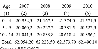
Table 1. Indonesian Population Projection Age 0-14 (2007-2010) (Thousand)
Age 2007 2008 2009 2010
(1) (2) (3) (4) (5)
0 - 4 20.952,5 21.167,5 21.374,0 21.571,5 5 - 9 20.060,2 20.227,2 20.381,5 20.522,5 10 - 14 21.041,5 20.833,8 20.618,2 20.396,1
Total 62.054,20 62.228,50 62.373,70 62.490,10 Source :BPS (2007)
Based on Ghana Standard Life Survey, Canagarajah and Coloumbe (1997) said that over 90% child labor came from rural living. They estimated that approximately 30.5% children age 7-14 are officially working. This number declined in 1998 become 22.4% and then increased in 1992 to become 28%. Most of child labor work in agricultural level. From the research in 1992, Canagarajah found that 66% from child labor are also school children. In Indonesia, if we saw data from Department of Social Services, we note that there is a declining number of Indonesian child labor in 1967-2000 but it is still show a significant
number. In 2006 about 1.6 million persons of Indonesian Population are recorded entering the labor market, which means there is 1.6 million children in Indonesia who are not going to school or working at the same time they go to school. Since school are an important aspect of human capital develop-ment, this case is a bad indicator.
In the first year of economic crisis in Indonesia, based on SAKERNAS data, pro-portion of children age 10-14 who economi-cally active increase to 7% in 1997 and 8% in 1998. Most of their motivation was, they want to help their family economic that fall due to crisis.
In fact parents realized that dropping children from school was harmful, in addition to lower skill acquisition, they also faced lower future income. But on the other hand, parents faced with the cost of schooling. This case is a symptom of the vicious circle of poverty, namely the situation when low level of saving resulted capital constraints, then restricts it, increase in productivity and it
Table 2. Numbers of People under Poverty Line and Child Labor 1976 – 1996 and 1997 – 2000 (%)
Under Poverty Line Child Age 10-14
Labor Force
Year Total
(%)
Total (Million)
ChildPopulation
(Million) Child Labor in
Labor Force
Age Cohort (%)
(1) (2) (3) (4) (5) (6)
1976 40,10 54,2 15,1 2,10 13,00
1980 28,00 42,3 17,6 1,98 11,27
1986 21,60 35,0 21,0 2,72 12,94
1990 15,10 27,2 21,5 2,24 10,41
1996 11,30 22,5 22,6 1,92 8,51
1998 Des. 24,20 49,5 21,7 1,79 7,91
1999 Feb. 23,50 48,4 - - -
1999 Aug. 18,20 37,5 20,9 1,52 6,96
2000 19,00 37,3 20,2 1,06 4,71
creates a persistent relationship of the poverty cycle. Throughout the crisis in 1998 and 1999,
Indonesian Central Bureau of Statistics (Biro
Pusat Statistik), with the assistance of UNICEF did a survey named the 'One hundred Village Survey'. This survey includes data from 12,000 households in 100 villages. One hundred villages were taken from 8 provinces in Indonesia. Let's see the result below, whether their data can be compared with previous data from SAKERNAS.
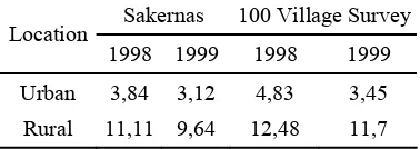
Table 3. Child Labor Age 10-14 Based on Sakernas and ‘100 Village Survey’ (%)
Sakernas 100 Village Survey
Location
1998 1999 1998 1999
Urban 3,84 3,12 4,83 3,45
Rural 11,11 9,64 12,48 11,7
Source : “100 village Survey” Data
The table above shows that both Sakernas and 100 Village Survey present a similar relative number of child labor. This number indicates that child labor in rural areas is three times greater than in urban areas and both sources show that there is a declining percentage of child labor from 1999 to 1998 in both environment. Although the number of Child Labor is greater in rural area than in urban area, but in a long term child workers will move to urban area for better living. They will migrate to places that give a bigger opportunity towards a better family’s econo-my. Most children who work in the informal sector in urban area are from the agrarian regions outside the modern sector, and usually they migrate by family decision that involve all family numbers including children and/or based on the children’s own decisions (Giani, 2006). Because of ethnic and geographical differences in Indonesia, study of labor mobility and internal migration pattern became very complex. This study is trying to explore that aspect while remembering that
Indonesian people have a very high viscosity for moving.
This research will try to prove that poverty is a main magnitude that motivates people to move from rural to urban. In the first section we will try to introduce the problem. In second section we will explain the relationship between migration, child labor and poverty. In section three we will see the data for the determinants. In section four we will introduce the methodology, in section five we will estimate the migration model. And we will conclude the research in section six.
MIGRATION, CHILD LABOR, AND POVERTY
Migration is an unavoidable problem in most of developing countries, due to lack of data, forecasting migration pattern is a very expensive and complex study. Because of declining job opportunities in rural areas people move to urban areas for increasing opportunities, hence many rapidly expanding Asian economies have seen increases in the rate of internal migration.
Empirical evidence proves that Indonesia is one of the developing countries with highest labor mobility. Labor mobility is long standing feature but recent rapid increases have attracted attention (ILO, 2004). There has also been increasing diversity in the types of movement and the profile of migrants. Census data for last 30 years show an increase in inter-provincial migration especially in the case of women.
(1969) offers a simple, but powerful hypo-thesis. The essential idea is that urban jobs are more attractive than rural employment, entry to the better urban activities is somehow constrained and search for urban jobs openings can be more effectively conducted in close geographical proximity. As a result, urban migration is induced as an investment in job search for the attractive, urban opportunities (Lucas, 1997).
Todaro’s model above was in part of response of observations on migration into Nairobi, Kenya. That same city prompted a path breaking ILO employment mission focusing considerable attention on the operations of the informal labor market (ILO, 1972). Fields in 1975 combines these two, remodeling Todaro’s formal sector job search, financed in part by participation in the infor-mal sector. In addition, Fields hypothesizes that even rural residents who conduct an urban job search from their rural base have some chance of finding an urban formal sector job, though their chances of success are lower than for persons who move into town to search (which is quite consistent with the essence of Todaro’s original model). Another realistic alternative is to allow risk aversion on behalf of migrants (Lucas, 1997). Suppose for instance that the objective of family is to
assign some portion of family members (ϕ)
such as to maximize
ρω (ϕ[w1-c] + [1-ϕ]wt) +
[1-ρ] ω(ϕ[w2-c] + [1-ϕ]wr) (1)
Where ρ is probability of obtaining a formal
sector urban job, ω is the family’s utility
function, w1 is urban formal sector wage, w2is
the urban informal sector wage, and wr is the
rural wage and c is cost of migrating. If the
utility function takes a simple logarithmic form, then using the first-order condition with respect to ϕ it can be shown that ϕ>0 if and only if
ρw1+[1- ρ]w2-c > wr (2)
it follows that when w2 = c = 0, equilibrium
with positive assignment of some family members to town in this case of risk aversion requires ρw1 > wr.
How about other research about poverty and internal migration? Some view revealed that migration can reduce poverty, inequality and contribute to economic growth and development, because of equality of wages that start when people from rural with lower wages move to urban area for wages hence the fact that over migration can come to bigger inequality, which means bigger poverty rate and bigger constrain on economic growth and development. This case is important in developing country especially for regional equality, unfortunately in Indonesia there has been no strong policy to control migration flow. People came to bigger cities in Indonesia independently without strict rules and they involve a number of family and friends to join the migration, and the things that happens next is the bigger cities will over populate, lack of decent living, came with more unemployment and create bigger disparity between whose rich and whose poor while rural area became more abandoned.
Rogers et. al.(2006) said in his research that forecasting migration pattern in Indonesia was very hard thing to do because of existence of large error in the model, but he count the migration propensity of people that move from east to west Indonesia region classified by age cohort. Like Mexico, much of recent changes in Indonesia are related to urbanization and rural to urban migration. Indonesian rural-out migrants, in general, target the larger cities as destination. As a result, the rural population in Indonesia has declined in absolute terms, and between 1980 and 2000, the percentage of population living in urban areas rose from 22% to nearly 42% (Rogers et. al., 2006).
than 0.03 (called labor force region shift) and this propensity decline for groups of age 20 or more, this analysis strengthen the previous assumption that not only people at productive age who move but also children. It means that relationship between migration and poverty also involve children as members of Rural-Urban Migrants. They skip school, live in harmful situation and unguaranteed future, not the environment that their children should be in.
DATA
The 2000 Population Census, which was done in June 2000, was the fifth census taken after the Independence of the Republic of Indonesia. The four previous censuses were taken in 1961, 1971, 1980, and 1990. There were improvements of many aspects from one census to the next, which include methodo-logy, concept, questionnaire design and covered areas. In the first four of Indonesian population censuses (1961, 1971, 1980, and 1990) a short form of questionnaire covered basic information such as age, sex and relation to the head of household used to enumerate households all over the country. On the other hand the long form questionnaire which
covered more detailed information (such as age, sex, place of birth, occupation, religion, educational attainment, migration status, ferti-lity and mortaferti-lity rate) was applied to collect data from a number of selected households. Therefore, the census result was published in two kinds of publication. The first was based on complete enumeration and the second was based on sample survey (BPS, 2000).
This study use Indonesian Census 2000 Data to estimate how many people leave their origin domicile for about 5 years in Java Region as the most crowded island in Indonesia, filtered with age and activities in destination and we measure population of child labor which migrates from another region. This study includes 110 region as observations. Because the model consists of two ways to count determinants of child labor migration (inflows and outflows migration) then the data are divided into two types of migration flows. The other determinants are collected from other data publication such as Central Bureau of Statistics (BPS) and
Bappenas (Indonesian National Planning Department). There is also an agglomeration variable to prove that urban-rural migration really happen with poverty causes. . Because Source : Rogers et. all (2006)
we assume that this migration is a long term phenomenon, some of data used are lagged for the estimation model.
The other determinants are Poverty with proxy Head Count Index (HCI) as a region characteristic of wealth that makes it easier to see how many people leave the rural areas as poles of poor regions. Minimum Regional Wages as characteristic of wealth in urban areas to prove that people really want to move interested by larger wage. Agglomeration as dummy variable that show whether a region agglomerate or not. Share and Constant Value in Manufacture sector as a variable that shows growth characteristics of urban areas that attract people to move. Literacy Rate as rural characteristic in growth of education. Sex Ratio of total Boys and Girls in each region. Ratio of Asset which describe people who have larger possibilities to move are usually people who have less asset in each region. Our migration model constrained with data inconsistency, we are focus on proving that migration of child labor move from rural that have a strength correlation with poverty to urban areas. Child Labor migration as a dependent variable of the model divided into outflows and inflows migration model. We use separate inflow and outflow model to observe the determinant of migration (described in outflow model), and the characteristic of destination on the inflow model that pull people to move to the destination.
Because of these data difficulties, we cannot get any further information about the specific regions where people want to move. We can only get the regions of origin in outflow model and the destination region in the inflow model. Hence this is not taken as a serious problem since we focus only in which regions have the largest magnitude of child labor migration
METHODOLOGY
This study will use spatial econometrics method. Regional economics has a very strong
correlation with spatial analysis, because in regional economics we analyze region as a space. Regional economy are spatially related with every economic activity, not limited to narrow purposes about production activity by firms, agriculture and mining, but encompass kinds of entrepreneurship, households and institution, both government and private. It refers to location in relationship with other economic activity, relationship closeness, concentration, spread, similarities, or differen-ces on spatial patterns. This discussion lead us to another general term such as inter regional analysis, micro geographic, zone, and location.
There are several reason for the use of geographical analysis in migration studies. The first is that the survey of characteristics on child labor may contain measurement errors. A bias may occur when researcher ignore wealth differences across region in the country. Several studies revealed the fact that rural child labor’s almost three times bigger than in urban areas, but we should not abandon the rational thought that in the long term they will migrate to urban areas in line with the decrease of land productivity in rural areas that pushes people to deeper poverty. The second reason is that poverty may have a spillover effect on the spread of child labor. Another problem that may arise when data have a locational component is that parameters in such a model are not homogenous over space but vary across different geographical locations. This is known as spatial hetero-geneity (Anselin, 1998).
repeated sampling. This gives rise to the need for alternative estimation approaches. Spatial heterogeneity violates the Gauss-Markov assumption that a single linear relationship varies as we move across the sample data observations. If the relationship with constant variance changes, alternative estimation is needed to successfully model this variation and draw appropriate inferences (LeSage: 1999a). As a more formal test, we calculate
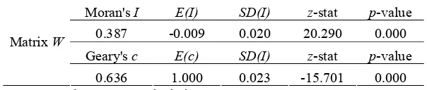
Moran’s I and Geary’s c statistics as two
common measures of spatial autocorrelation. The null hypothesis is no spatial dependence. If I is greater (smaller) than its expected value,
E(I), the overall distribution of Migration is
characterized by positive (negative) spatial dependence. If c is greater (smaller) than its expected value, E(c) the overall distribution of Migration characterized by positive (negative) spatial dependence. The statistical inference is computed on the basis of z-statistics.
Table 4 shows that Moran’s I statistics are
greater than -0.005 with highly positive z
-values, while Geary’s c statistic is smaller than one with highly negative z-values. This result indicates positive dependence of the migration among regions. Following Tobbler’s First Law of Geography, we employ spatial weighting matrix using row standardized continues distance decay function, whereas the distance measurements were taken from the district’s centroid points. The spatial weight that we use (W) is based on kilometer-converted Euclidean Distance (dij) between districts (i and j) on the sphere:
|) | cos cos (cos
) sin n arccos[(si
δγ φ φ
φ φ
j i
j i ij
d = +
(3)
Where i and j are the centroid’s latitude of district i and j, respectively |δγ|denotes the absolute value of the difference in longitude and latitude between i and j. A spatial weights
matrix W is a N by N nonnegative matrix,
which expresses for each region (row) those regions (columns) that belong to its neigh-borhood set as nonzero elements. By convention, the diagonal elements of weight matrix are set to zero, since no regions can be viewed as its own neighbor. For the ease of interpretation, it is common practice to
normalize W such that the elements of each
row sum to one. Since W is nonnegative, this
ensures that all weights can be interpreted as an averaging of neighboring values.
There is two kinds of spatial regression model that usually use on spatial analysis. The first is Spatial Auto Regressive (SAR) and the second is Spatial Error Model (SEM) respectively:
a) SAR (Spatial Auto Regressive)
This model focuses on spillover effect existence. This model tries to estimate whether “x” variable in a region affect or affected by “x” variable in the neighbor region. The model noted as :
∈ + + = Wy Xij
y ρ (4)
Table 4. Moran’s I and Geary’s c for Migration Model
Moran's I E(I) SD(I) z-stat p-value
0.387 -0.009 0.020 20.290 0.000
Geary's c E(c) SD(I) z-stat p-value
Matrix W
0.636 1.000 0.023 -15.701 0.000
Where ρ is a spatial autoregressive
coefficient, and ∈ is a vector of error terms
and the other notation are the independent and dependent variables. Unlike what holds for time series counterpart of this model, the
spatial lag term Wy is correlated with the
disturbances. This can be seen on a reduce form :
In which inverse can be expanded into an infinite series including both the explanatory variables and the error terms at all location (the spatial multiplier). Consequently, the spatial lag term must be treated as an endogenous variable and proper estimation methods must account for this endogeneity while OLS will be biased and inconsistent due to the simultaneity bias (Anselin, 1988).
b) Spatial Error Model (SEM)
Spatial Error model estimates correction model with large error. A spatial model error is a special case of regression with non-spherical error term, in which the off-diagonal elements of the covariance matrix express the structure of spatial dependence. Consequently, OLS remain unbiased, but it is no longer efficient and the classical estimator for standard errors will be biased. In the form of spatial Durbin or spatial common factor model (Anselin, 1988), the Spatial Error Model is
u
Which is spatial lag model with an additional set of spatially lagged exogenous variables
(WX) and set of “k” nonlinear (common
factor) constrains on the coefficient (the pro-duct of the spatial autoregressive coefficient β
should equal the negative of the coefficient of
WX. The similarity between the error model
and the “pure” spatial lag model will complicate specification testing in practice, since tests designed for a spatial lag alternative will also have power against a spatial error alternative will also have power against a spatial error alternative, and vice versa.
MODEL ESTIMATION
After the migration model in Java is estimated, surprising numbers reveal a lot of stories, both inflow migration model and outflow migration model use two classifi-cation of age which define a different point of view of age of Child Labor. United Nation General Assembly in 1989 stated that a person called children when they are still under 18 years old. But in the Central Bureau of Statistics (BPS) classified a person is in the unproductive age (Child) when he/she still under 15 years old. In this paper both classification are estimated, gave different size of coefficient but still have similarity in the sign.
The first model of inflow migration for children under 15 in Java use agglomeration indicator variable as a dummy variable, 1 if the region was a part of an agglomeration and 0 if the region was not a part of an
agglome-ration (aglmr), natural logarithm of constant
manufacture share to national income (Ln(comanf)), and natural logarithm of
regional minimum wages (Ln(UMR)) as a
determinant, noted first as an OLS model:
i
The inflow model for child under 18 noted as:
Different from the first inflow model, in order to avoid heteroscedasticity problem because of the same pattern between error and constant manufacture value in inflow mi-gration model for children under 18, we use share of manufacture sector output to national income as determinants. Although we have two different definition of the determinants, but in the end we have same interpretation to recognize the urban characteristics through manufacture sector.
The second model is outflow migration model, which use the same classification age as the inflow model. For outflow migration model of children under 15, we use poverty rate relative to Jakarta, this determinants was used in order to compare poverty rate in rural area with urban area, in Indonesia, for benchmarking purpose, we use as it was the
biggest urban agglomeration in Java (Povji),
literacy rate as a characteristics of origin region which we assume as a rural area (Literi), sex ratio between total male and female in a region to show whether compo-sition of male over female determine mobility of the people in a region (Sxrati), and ratio of asset owned by people at a region i (Raseti) was used as a determinant under assumption that family with a bigger asset will have a less probability to move.
The outflow model for children aged under 15 and 18 respectively noted as:
i
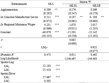
And the model estimation shows the robustness of the model. Let us see the estimation of children age 15 inflow migration
model using OLS and spatial regression. The determination of inflow migration model (child labor under 15) means variable which causes people to go into the urban area, this model shows that there is positive relationship between child labor inflow migration and agglomeration, this is reveals a signal that urban area attract not only people at productive age but also children to enter the labor market; this variable shows the right sign, when the city agglomerate the inflow migration come larger, and the variable is robust even when the estimation model has been changed into another form of inflow model. And there is also positive relationship between child labor inflow migration with constant value of manufacture sector, indi-cating that child labor come to urban for this sector; the coefficient shows the right sign also, because we assume that people that go to urban areas, rationally thinks that region that have dominant manufacture sector with its labor incentives production processes gives bigger opportunity at job vacancy.
Minimum Regional Wages also shows a robust and consistent sign of relationship to inflow migration, along with other variables that showed the right sign, this variable also appropriate with the theory that people migrate to urban areas based on expected value of wages, regional minimum wages as a standard of wages in a region will affect personal expected of wages (Todaro, 1969). The higher the minimum regional wages determined by the government, the larger the labor’s expectations. The spatial regression shows that Lagrange Multiplier Value on Spatial Lag Method even is even higher than those for Spatial Error Method, and its also has
significant ρ value, it means that there is
spatial autocorrelation in the model, that Urban areas pull rural people to moves.
coefficient (ρ) of this model shows higher
number than in spatial error coefficient (λ).
This means that there is no big difference in what motivates migration decisions in both models, higher growth in destination are, bigger opportunities, also larger magnitudes areas that pull people to migrate. This also showed the robustness of the models.
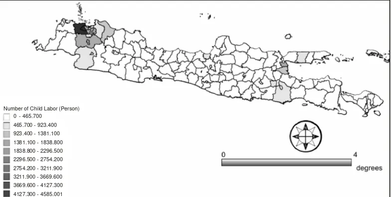
We can also see which region are the has magnitude in the inflow migration model, we can see the map of Java below (Picture 2). The map projected numbers of inflow in each region indicated by the color. Red color indicates higher number of child labor migration inflow in each region. The map for child labor under 15 years old show that the urban area with largest magnitude in Java is around Tangerang and the region around Jakarta, also Depok, and Bekasi. Tangerang is
the largest manufacture industry region in Java, noted by the amount of manufacture share to national income that is equal to 58%.
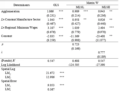
This is the answer why this region became the determinant for people to migrate. And we can also see one of the region that pull people in East Java is the region around Surabaya, the third largest city in Java after Bandung and Jakarta, also a manufacturing industries region, giving 35% in share of manufacture sector compared to total output. This picture strengthens our empirical result. The pictures draw by software Quantum GIS Version 1.0.2.0. The similarities observed in Migration Inflow Model for children under 18 years old. Tangerang still holds the biggest magnitude for child labor migration.
Number of Child Labor (Person) 0 - 465.700
465.700 - 923.400 923.400 - 1381.100 1381.100 - 1838.800 1838.800 - 2296.500 2296.500 - 2754.200 2754.200 - 3211.900 3211.900 - 3669.600 3669.600 - 4127.300 4127.300 - 4585.001
Source : Author's Projection Using Data from Indonesian Sensus 2000
Number of Child Labor (Person) 0 - 1500
1500.1 - 3000 3000.1 - 4500 4500.1 - 6000 6000.1 - 7500 7500.1 - 9000 9000.1 - 10500 10500.1 - 12000 12000.1 - 13500 13500.1 - 16000
Source : Author's Projection Using Data from Indonesian Sensus 2000
Figure 3. Map Inflow for Children Under 18 Years Old in Java Island
Table 5. Estimation Inflow Migration Model for Child Labor Age Under 15 Years Old in Java
Matrix W Determinants OLS
MLSL MLSE
Agglomeration 0.389) ** 0.276) 0.269)
(0.292) (0.247) (0.278)
Ln Constant Manufacture Sector 0.211) 0.187) ** 0. 188) **
(0.072) ***
(0.061) (0.063)
Ln Regional Minimum Wages 4.231) *** 1.078) 2.017)
(0.866) (0.811) (1.235)
Constant -49.970) *** -15.201) -22.142)
(10.235) (9.556) (15.192)
ρ 0.885)
(0.098)
λ LMρ 0.922)
(0.077)
(Pseudo) R2 0.473) 0.611) 0.462)
Log Likelihood -1140.467) -144.493)
Spatial Lag
LMρ 52.183) ***
LMγρ 25.418) ***
Spatial Error
LMλ 27.067) ***
LMγλ 0.302)
Table 6. Estimation Inflow Migration Model for Child Labor Age Under 18 Years Old in Java
Matrix W
Determinants OLS
MLSL MLSE
Agglomeration 1.066 *** 0.909) *** 0.943) **
(0.231) (0.214) (0.236)
Ln Constant Manufacture Sector 1.043) 0.958) ** 0.926) **
(0.467) ***
(0.427) (0.440)
Ln Regional Minimum Wages 3.107) *** 1.039) 2.404) ***
(0.676) (0.779) (0.970)
Constant -2.035) *** -11.369) -23.408) **
(8.259) (8.908) (11.877)
ρ 0.723)
(0.166)
λ 0.777)
(0.189)
(Pseudo) R2 0.547) 0.608) 0.547)
Log Likelihood -124.505) -27.390)
Spatial Lag
LMρ 21.672) ***
LMγρ 12.986) ***
Spatial Error
LMλ 9.053) ***
LMγλ 0.367)
Standard error in brackets; ***,**,and *: significant at 1%,5%, and 10%
Outflow migration model tells different story. Outflow migration model tells us what determines child labor to move from the origin
destination, our ex-ante assumption reveals
that high poverty and low wealth being the biggest reasons to move. This outflow migration models also divided into two classifications of age, for child under 15 and under 18 years old. In outflow migration model we use poverty rate relative to Jakarta just like in the inflow model, this determinants was used in order to compare poverty rate in rural area with urban area, in Indonesia, for benchmarking purpose, we use as it was the
biggest urban agglomeration in Java (Povji),
also literacy rate (Literi) as education indicator in rural area, we assume that the higher the literacy rate in a region is, the less people will
migrate, and we use sex ratio (Sxrati) to
analyze the ratio between male and female in a region, and ratio of asset between who own
house and rent house (Raseti) as an indicator
increased, urban needs more labor with at least ability to read.
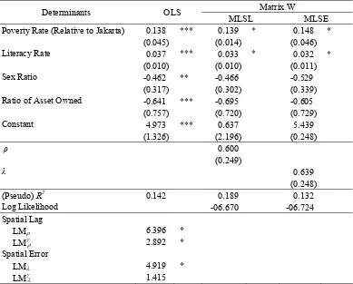
Negative relationship between sex ratio and child labor migration, indicate that male tend to move more than female, some of female prefer to stay at their origin than migrate to urban for job. And the empirical result shows negative relationship between ratio of asset owned, which reinforce our assumption.
The under 18 outflow migration also shows similar numbers and same sign of the coefficients. Both spatial regression show that spatial lag is significant. There is spatial
dependence in spatial regression model since Moran’s I coefficient has positive sign. This outflow model also shows the robustness of the models using different age classification.
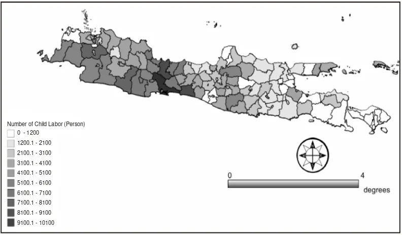
And what does the map say about outflow data?, The map implies the the peripherial area in Java Island is the biggest supplier of child labor to urban areas. In West Java, Southern Areas one filled with red color such as Pameungpeuk, South Cianjur, and Ciamis, also Southern Central Java such as Kebumen, Magelang, and Banyumas. This fact confirm with our hypothesis which states that child labor moves from periphery areas.
Number of Child Labor (Person) 0 - 1200
1200.1 - 2100
2100.1 - 3100
3100.1 - 4100
4100.1 - 5100
5100.1 - 6100
6100.1 - 7100
7100.1 - 8100
8100.1 - 9100
9100.1 - 10100
Source : Author's Projection Using Data from Indonesian Sensus 2000
Number of Child Labor (Person) 0 - 2300
2300.1 - 4100 4100.1 - 5800 5800.1 - 7600 7600.1 - 9400 9400.1 - 11000 11000.1 - 13000 13000.1 - 14500 14500.1 - 16400 16400.1 - 18500
Source : Author's Projection Using Data from Indonesian Sensus 2000
Figure 5. Outflow Map For Outflow Migration for Children Under 18 Years Old
Table 7. Estimation of Outflow Migration Model for Child Under 15 Years Old in Java Island
Matrix W
Determinants OLS
MLSL MLSE
Poverty Rate (Relative to Jakarta) 0.138) *** 0.139) * 0.148) *
(0.045) (0.014) (0.046)
Literacy Rate 0.037) 0.033) * 0.032) *
(0.010) ***
(0.010) (0.011)
Sex Ratio -0.462) ** -0.466) -0.529)
(0.317) (0.302) (0.339)
Ratio of Asset Owned -0.641) *** -0.695) -0.605)
(0.757) (0.720) (0.729)
Constant 4.973) *** 0.637) 5.439)
(1.326) (2.196) (0.248)
ρ 0.600)
(0.249)
λ 0.639)
(0.248)
(Pseudo) R2 0.142) 0.189) 0.132)
Log Likelihood -06.670) -06.724)
Spatial Lag
LMρ 6.396) *
LMγρ 2.892) *
Spatial Error
LMλ 4.919) *
LMγλ 1.415)
Table 8. Estimation of Outflow Migration Model For Child Under 18 Years Old in Java Island
Matrix W
Determinants OLS
MLSL MLSE
Poverty Rate (Relative to Jakarta) 0.130) *** 0.132) ** 0.138) *
(0.043) (0.041) (0.044)
Literacy Rate 0.032) 0.029) 0.028) *
(0.001) ***
(0.001) (0.010)
Sex Ratio -0.294) ** -0.324) -0.367)
(0.302) (0.290) (0.323)
Ratio of Asset Owned -1.086) ** -1.096) -1.016)
(0.721) (0.691) (0.701)
Constant 6.429) *** 2.192) 6.726)
(1.262) (2.511) (1.291)
ρ 0.522)
(0.271)
λ 0.554)
(0.284)
(Pseudo) R2 0.132) 0.162) 0.116)
Log Likelihood -101.968) -102.121)
Spatial Lag
LMρ 4.232) **
LMγρ 3.608) *
Spatial Error
LMλ 2.865) *
LMγλ 2.240)
Standard error in brackets; ***,**,and *: significant at 1%,5%, and 10%
CONCLUSION
Migration pattern in Java Island has proved the hypothesis that migration from rural to urban was happened for reasons such as low wealth, high poverty, and high wages in urban areas, influence people to migrate. There is spatial dependence on migration among regions which is robust to changes of the model’s dependent variable definition. Both inflow and outflow model estimation results implies the right sign. The model shows that agglomeration, minimum regional wages, and value of manufacture sector influence the inflow migration into urban area,
Our government has made so many policy to control growth of Indonesian population, such as family planning and more rules about transmigration, but somehow government ignored this pattern of migration which include child labor as member of the migrants. Rural development really needed in order to decrease stimulation of migration push; also revision of labor policy so there is a strong restriction for children to enter the labor market. And the most important things to done, increase the development of education, because we believe that in a long term well educated children will result better future for Indonesia.
REFERENCES
Todaro, Michael P., 2003. Pembangunan
Ekonomi Dunia Ketiga (The Development
of Third World Country). Erlangga.
Indonesia.
Rogers, Andrei et. al., 2007. “Inferring migration flow from the migration propensities of infants: Mexico and
Indonesia”. The Annals of Regional
Science 41(1), 443-465
Giani, L., 2006, “Migration and Education : Child Migrants in Bangladesh”, Susex Migration Working Paper 2006-33. United Kingdom: University of Susex.
Anselin, Luc., 1988, Spatial Econometrics:
Methods and Models, Boston: Kluwer Academic Publisher.
Pitriyan, Pipit, 2006, “The Impact of Child
Labor on Child’s Education: The Case of
Indonesia”. Working Papers of Economic
Development Studies. Padjadjaran Univer-sity, Bandung.
Suryahadi, Asep et., 2005, “What Happened to Child Labor in Indonesia During Crisis? The Tradeoff Between School and Work”,
SMERU Working Paper. Jakarta: SMERU Research Institute.
LeSage, James P., 2004, A Family of
Geo-graphically Weighted Regression Models
in elin, Luc., Florax, Raymond J.G.M.,
and Serge J. Rey (Eds.), 2004, Advances
in Spatial Econometrics: Methodology Tools and Applications, Springer Series in Advances in Spatial Science, Springerlink.
Tobler, W. R., 1970, A Computer Movie
Simulating Urban Growth in the Detroit Region, Economic Geography (Supple-ment: Proceedings. International
Geogra-phical Union). Commission on
Quantita-tive Methods, 46(2), 234-240.
Brown, Annete N., 1997, “The Economic Determinants of Internal Migration Flows
in Russia During Transisition”. The
Davidson Institutes Working Paper Series. Paper 1997-89. Michigan: William Davidson Institute.
Lucas, Robert E.B., 1997, Handbook of
Family and Economics Internal Migration in Developing Countries, ed. M.R. Rosenzweig and o. Stark. Boston Univer-sity, Elseviere-Science Press, Boston : 721-78
Fields, G.S., 1975, “Rural-urban migration, urban unemployment and underemploy-ment, and job-search activity In LDCs”,
Journal of Development Economics, 2, 165-187.
Stiglitz, J.E., 1974, “Alternative theories of wage determination and unemployment in LDCs: the labor turnover model”,
Quarterly Journal of Economics, 88, 194-227.
Seldadyo, Harry, 2007, “Geography and Governance: Does Space Matter?”,