Genetic differentiation of water buffalo
(Bubalus bubalis) populations in China, Nepal
and South East Asia: inferences on the region of
domestication of the swamp buffalo
Article
in
Animal Genetics · August 2011
Impact Factor: 2.21 · DOI: 10.1111/j.1365-2052.2010.02166.x · Source: PubMed
CITATIONS
9
READS
178
3 authors:
Ying Zhang
Chinese Academy of Sciences
144 PUBLICATIONS2,077
CITATIONSSEE PROFILE
Dianne M Vankan
University of Queensland
47 PUBLICATIONS229
CITATIONSSEE PROFILE
James Stuart F Barker
University of New England (Australia)
265PUBLICATIONS4,844CITATIONS
SEE PROFILE
Genetic differentiation of water buffalo (
Bubalus bubalis
)
populations in China, Nepal and south-east Asia: inferences on the
region of domestication of the swamp buffalo
Y. Zhang*, D. Vankan
†, Y. Zhang* and J. S. F. Barker
‡*Department of Animal Genetics and Breeding, College of Animal Science and Technology, China Agricultural University, Beijing 100193, China.†The School of Veterinary Science, The University of Queensland, Gatton Campus QLD 4343, Australia.‡School of Environmental and Rural Science, University of New England, Armidale, NSW 2351, Australia
Summary Data from three published studies of genetic variation at 18 microsatellite loci in water buffalo populations in China (18 swamp type, two river type), Nepal (one wild, one domestic river, one hybrid) and south-east Asia (eight swamp, three river) were combined so as to gain a broader understanding of genetic relationships among the populations and their demographic history. Mean numbers of alleles and expected heterozygosities were signifi-cantly different among populations. Estimates ofh(a measure of population differentiation) were significant among the swamp populations for all loci and among the river populations for most loci. Differentiation among the Chinese swamp populations (which was due pri-marily to just one population) was much less than among the south-east Asian. The Nepal wild animals, phenotypically swamp type but genetically like river type, are significantly different from all the domestic river populations and presumably represent the ancestral
Bubalus arnee(possibly with some river-type introgression). Relationships among the swamp
populations (DA genetic distances, principal component analysis and STRUCTURE analyses)
show the south-east Asian populations separated into two groups by the Chinese popula-tions. Given these relationships and the patterns of genetic variability, we postulate that the swamp buffalo was domesticated in the region of the far south of China, northern Thailand and Indochina. Following domestication, it spread south through peninsular Malaysia to Sumatra, Java and Sulawesi, and north through China, and then to Taiwan, the Philippines and Borneo.
KeywordsBubalus arnee, domestication, microsatellite, population differentiation, river buffalo, swamp buffalo.
Introduction
The world population of water buffalo in 2008 was reported (http://faostat.fao.org, 26 May 2010) as 181 million, but this did not distinguish between numbers of the two types – river and swamp. The swamp and river buffalo are differ-entiated on morphological and behavioural criteria and are well known to be genetically distinct, based on chromosome number and allozyme and microsatellite genotype frequen-cies. Their endemic distributions are parapatric, with the
swamp type found throughout south-east Asia, from Assam and Nepal in the west to the Yangtse valley of China, while the river type is native to the Indian subcontinent, but has spread west to the Balkans, Italy and Egypt within historical times (Cockrill 1974). The water buffalo has been described as under-utilized (NRC 1981), even though more people in the world depend on this species than on any other domestic animal species (FAO 2000).ÔUnder-utilizedÕin this context apparently meansÔnot improvedÕ, or not subject to breeding programmes in the case of the swamp buffalo, and also refers to opportunities for the wider use of both swamp and river buffalo in regions outside south-east Asia and the Indian subcontinent.
Breeding programmes and optimal utilization require knowledge of genetic variability, that is, diversity within and among breeds and populations. Furthermore, data on
Address for correspondence
J. S. F. Barker, School of Environmental and Rural Science, University of New England, Armidale, NSW 2351, Australia.
E-mail: [email protected]
the magnitude of genetic differentiation and genetic rela-tionships among breeds and populations are necessary for defining the best approaches to the conservation of genetic resources.
Our previous studies of genetic diversity have been pri-marily of swamp buffalo populations in south-east Asia (Barkeret al.1997a,b) and China (Zhanget al.2007), and Nepalese populations of wild buffalo and domestic river buffalo (Flamand et al. 2003). By combining these three previously published data sets, our interest is in further understanding the relationships among the populations and their demographic history, and possibly the origin and domestication of the swamp type of water buffalo.
Materials and methods
We have used data from three of our published studies on microsatellite genetic variation in water buffalo populations: from Barkeret al. 1997b, 21 loci in 11 south-east Asian and Australian (hereafter SE Asian) populations (eight swamp, three river); from Zhanget al.2007, 30 loci in 20 Chinese populations (18 swamp, two river); and from
Fla-mand et al. 2003, 10 loci in three Nepalese populations
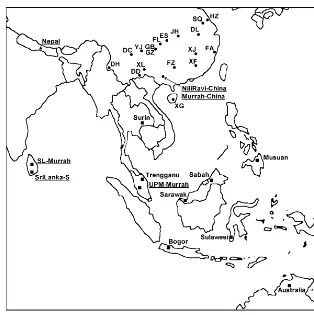
(wild, domestic river and hybrid) (see Fig. 1 for a map showing all population locations). For the first two data sets, 20 loci were in common, and the ten used for the Nepalese populations were included in these. DNA was retained for
the Nepal samples, and the other ten loci were genotyped in the same laboratory as for the first ten. As the initial genotyping had been performed in three different laborato-ries, we used two approaches to standardize genotype scoring. We compared allele frequency distributions sepa-rately for swamp and river buffalo for each locus. We genotyped a selected set of 30 samples from the Chinese populations in the laboratory where the Nepal samples were assayed and utilized the same protocols. These 30 were selected to provide a range of alleles for each of the 20 loci. Allele size nomenclature was entirely consistent for five loci and differed by one bp for nine loci and by two bp for two loci. For two loci, shorter alleles were consistent, but the longest alleles differed by one or by two bp. Allele size nomenclature of one or other data set was changed as necessary to match across all data sets. For two loci (CSSM033 and CSSM047), genotyping differences between the data sets could not be simply reconciled, and these loci were deleted. Thus, all analyses of the 34 populations here have used data on 18 loci.
Reassignment of Nepal animals
The Nepalese animals comprised putative wild water buffalo
(Bubalus arnee) and putative hybrids (classified
phenotypi-cally), as well as animals identified by their owners as domestic river type. Given the genotypic data for the ten
Figure 1 Map showing the locations of all sampled populations (nSE Asian populations,
microsatellites, Flamand et al.(2003) used genetic admix-ture analysis and population assignment to reassign ani-mals as identified genetically to wild, hybrid or domestic types. One of the loci used in that study (CSSM033) was omitted in the present study; results for the additional nine loci were added to the data set; and the analysis was per-formed again. We used the methods of Pritchard et al.
(2000) and Hubisz et al. (2009), as implemented in the programSTRUCTURE2.3.1. This method is a Bayesian
cluster-ing approach uscluster-ing multilocus genotypes to infer population structure and to assign individuals to populations. It assumes Hardy–Weinberg equilibrium and linkage equilib-rium between loci within each population. STRUCTURE2.3.1
can allow for the correlations between linked loci that arise in admixed populations. However, this requires data on the relative positions of the markers, which are not available for our microsatellites. We used the estimated pairwise gametic disequilibrium (see below) to determine whether back-ground gametic disequilibrium is likely to increase the probability of detecting spurious clustering (Kaeuffer et al.
2007).
Individuals were initially assigned as wild, hybrid or domestic based on the previous analysis using ten loci. We used the admixture model and the option of correlated allele frequencies, with default parameters, except that the pre-defined populations were used as prior. A burn-in period of 500 000 steps was used, followed by 300 000 Markov chain Monte Carlo (MCMC) replicates.
Allele frequency, heterozygosity and gametic disequilibrium
Genotype and allele frequencies were estimated using
GENEPOP Version 3.4 (Raymond & Rousset 1995) (GENEPOP
data file for all 34 populations available as Table S1), and alleles per locus and observed and expected heterozygosity (gene diversity) usingGENECLASS2(Piryet al.2004). Tests for
deviations from Hardy–Weinberg equilibrium were per-formed using the exact tests ofGENEPOP(default values for
the Markov chain method). Significance levels for each test were determined by applying the sequential Bonferroni procedure (Hochberg 1988; Lessios 1992) over loci within each population to the probability estimates calculated by
GENEPOP. The allelic richness for each population was
esti-mated usingFSTAT2.9.3 (Goudet 2001), based on the
mini-mum sample size of the UPM-Murrah population. The number of alleles per locus and observed and expected heterozygosity were compared among populations using the Kruskal–Wallis non-parametric test (Sokal & Rohlf 1981).
Pairwise gametic disequilibria (LD) between loci within each population were estimated using the MCLD program
(Zaykinet al.2008). The probability value for each test was evaluated using both theT2test statistic (Zaykinet al.2008)
and a Monte Carlo (permutation) P-value. These gave similar results; the results presented here use the latter
approach. Significance levels for each test were determined by applying the sequential Bonferroni procedure (Hochberg 1988; Lessios 1992) over locus pairs within each popula-tion to the estimated P-values. In addition, we considered the percentage of locus pairs that had P-values <0.05, for each population. As 5% of the pairwise LD is expected by chance to be significant, higher percentages indicate more LD than expected (Schuget al.2007).
Population differentiation and relationships
Population differentiation and relationships may be biased if some loci are under selection. We have used a method (Excoffier et al. 2009) implemented in Arlequin3.5 for the detection of selection in a hierarchically structured popu-lation. Populations were grouped according to the structure defined by the initial phylogenetic analysis (see Results, Fig. 2) as (i) Chinese swamp populations (except DH), (ii) DH, (iii) Musuan, Sabah and Sawawak, (iv) Surin, Treng-ganu, Bogor, Sulawesi and Australia, (v) Chinese river populations, (vi) Nepal domestic, Sri Lanka and Malaysia river populations, (vii) Nepal wild and hybrid. Following Excoffier et al. (2009), we assumed the SMM model, used
qST, and the simulation parameters were 50 groups and
100 demes per group, with 50 000 simulations.
F-statistics (Weir & Cockerham 1984) and their signifi-cance were determined using FSTATVersion 2.9.3 (Goudet
2001), not assuming Hardy–Weinberg equilibrium and with 5000 iterations. Genetic relationships among the populations were studied using three complementary methods. Genetic distances (the DA distance of Nei et al.
1983) were obtained using theDISPANprogram (Ota 1993),
and a dendrogram of genetic relationships among the pop-ulations was constructed as a neighbour-joining tree (Sai-tou & Nei 1987) using POPTREE2(Takezaki et al.2010). In addition, SPLITSTREE4(Huson 1998) was used to produce a
neighbour-net plot of population relationships. Principal component analysis (PCA) of gene frequency data was
performed using the PCAGEN program (Goudet 1999).
Finally, we again used STRUCTURE2.3.1 as above (with
sam-pling locations as prior). Following preliminary testing, we used a burn-in of 100 000 iterations followed by 100 000 MCMC replicates. Structure runs performed for different values of the number of clusters (K) were evaluated using the model choice criterion Ln P(D), which is the posterior probability of the data for a given K. The true number of clusters is commonly inferred as that giving the maximal value of Ln P(D), but Pritchard et al. (2009) warn that Ln P(D) may continue to increase beyond theÔtrueÕvalue of
K. The standard deviation of Ln P(D) was estimated from five replicate runs for each value ofK, but for any givenK
value, the run with maximum Ln P(D) was used for assignments and for defining the appropriateKfrom the plot of Ln P(D) on K. We also used the DKmethod of Evanno
of the structure in our data considers both theÔvalues ofK
that capture most of the structure in the data and that seem biologically sensibleÕ(Pritchardet al.2009) and the modal value of the distribution ofDK (Evanno et al. 2005). The output from STRUCTURE was visualized using the DISTRUCT
program (Rosenberg 2004).
Results
Reassignment of Nepal animals
For theSTRUCTUREanalysis, assignment was done using the
prior population information (option USEPOPINFO = 1). That is, we assumed that each individual belongs with high probability to the group to which it was classified (wild, hybrid or domestic), but allowing some probability that it has some ancestry from the other groups. We have taken a value of 0.9 as a cut-off point, i.e. any animal classified to its pre-assigned cluster with probability value (q)‡0.9 was
accepted to that cluster, while if q< 0.9, the animal was assigned to the most probable of the other two clusters. Five individuals were reassigned: one wild to hybrid, one hybrid to wild, two hybrid to domestic and one domestic to hybrid; these were confirmed in a furtherSTRUCTURErun (Table 1). Finally, an analysis was performed with prior information on the wild and domestic animals only, so as to infer the ancestry of the presumed hybrid individuals. Probabilities of wild ancestry for the hybrids ranged from 0.255 to 0.329.
Genetic variability
The number of alleles per locus ranged from four (HMH1R) to 17 (CSRM060). All but four loci (CSSM038, CSSM045, BRN and HMH1R) were polymorphic in all populations (allele frequencies are available in Table S2). For CSSM045 and HMH1R, all the Chinese populations (except those in the south-west) and Sabah and Sarawak were fixed for the allele that was most common in the other swamp popula-tions. Sarawak was monomorphic also for CSSM038, and BRN and Sabah were monomorphic for CSSM038. Average genetic diversity (Nei 1973) over all loci was 0.672, and for individual loci, average genetic diversities ranged from 0.052 (HMH1R) to 0.880 (CSSM019). Twenty-six private alleles were identified in 14 populations, and of these, five were unique to DH and four to Surin. We also found one allele at CSSM045 that was unique to the wild and hybrid
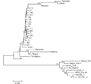
Figure 2.Dendrogram of relationships among all populations, usingDAgenetic distances and the neighbour-joining method of clustering. Numbers on the nodes are percentage bootstrap values (only those >50) from 1000 replications of resampled loci.
Table 1 Average inferred ancestry probabilities for each of the three Nepal groups – wild, hybrid and domestic water buffalo.
Average estimated ancestry
Population No. individuals Wild Hybrid Domestic
Wild 8 0.934 0.019 0.047
Hybrid 15 0.251 0.385 0.364
Nepal populations (frequencies of 0.125 and 0.033, respectively) and one at CSSM061 that occurred only in the three Nepal populations (frequencies of 0.125, 0.067 and 0.023 in wild, hybrid and domestic, respectively).
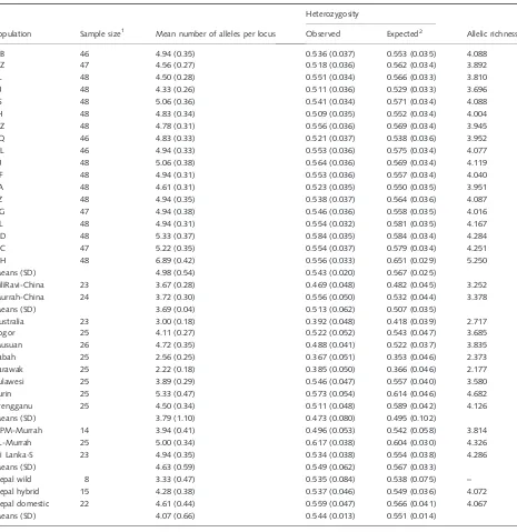
The populations, sample sizes and measures of genetic variability for each population are given in Table 2. The mean numbers of alleles per locus were significantly differ-ent among all populations (P< 0.0001), among the SE Asian populations (P< 0.0001) and among the river (including Nepal) populations (P= 0.013), but not among the Chinese swamp populations. Differences among the SE
Asian populations are due primarily to lower values for Australia, Sabah and Sarawak. The mean number of alleles for the other five SE Asian populations is not significantly different from the mean for the Chinese swamp populations. Differences among the river populations are due primarily to lower values for the Chinese Nili Ravi and Murrah, and the Nepal wild. Differences among populations for expected heterozygosity (He) were essentially the same as for number
of alleles, except that differences among the river popula-tions were not significant. Observed heterozygosities were not significantly different among all 34 populations.
Table 2Sample size and genetic variability measures (standard errors in parentheses) for each population.
Population Sample size1 Mean number of alleles per locus
Heterozygosity
Allelic richness Observed Expected2
GB 46 4.94 (0.35) 0.536 (0.037) 0.553 (0.035) 4.088
GZ 47 4.56 (0.27) 0.518 (0.036) 0.562 (0.034) 3.892
FL 48 4.50 (0.28) 0.551 (0.034) 0.566 (0.033) 3.810
YJ 48 4.33 (0.26) 0.511 (0.036) 0.529 (0.033) 3.696
ES 48 5.06 (0.36) 0.541 (0.034) 0.571 (0.034) 4.088
JH 48 4.83 (0.34) 0.509 (0.035) 0.552 (0.034) 4.004
HZ 48 4.78 (0.31) 0.556 (0.036) 0.569 (0.034) 3.945
SQ 46 4.83 (0.33) 0.521 (0.037) 0.538 (0.036) 3.952
DL 46 4.94 (0.33) 0.553 (0.036) 0.575 (0.034) 4.077
XJ 48 5.06 (0.38) 0.564 (0.036) 0.569 (0.034) 4.119
XF 48 4.94 (0.31) 0.553 (0.036) 0.557 (0.034) 4.040
FA 48 4.61 (0.31) 0.523 (0.035) 0.550 (0.035) 3.951
FZ 48 4.94 (0.35) 0.538 (0.037) 0.564 (0.036) 4.087
XG 47 4.94 (0.38) 0.546 (0.036) 0.558 (0.035) 4.016
XL 48 4.94 (0.31) 0.554 (0.032) 0.581 (0.035) 4.167
DD 48 5.33 (0.37) 0.584 (0.035) 0.584 (0.034) 4.284
DC 47 5.22 (0.35) 0.554 (0.037) 0.579 (0.034) 4.251
DH 48 6.89 (0.42) 0.556 (0.033) 0.651 (0.029) 5.250
Means (SD) 4.98 (0.54) 0.543 (0.020) 0.567 (0.025)
NiliRavi-China 23 3.67 (0.28) 0.469 (0.048) 0.482 (0.045) 3.252
Murrah-China 24 3.72 (0.30) 0.556 (0.050) 0.532 (0.044) 3.378
Means (SD) 3.69 (0.04) 0.513 (0.062) 0.507 (0.035)
Australia 23 3.00 (0.18) 0.392 (0.048) 0.418 (0.039) 2.717
Bogor 25 4.11 (0.27) 0.522 (0.052) 0.543 (0.047) 3.685
Musuan 26 4.72 (0.35) 0.488 (0.041) 0.522 (0.037) 3.835
Sabah 25 2.56 (0.25) 0.367 (0.051) 0.353 (0.046) 2.373
Sarawak 25 2.22 (0.18) 0.385 (0.050) 0.366 (0.046) 2.177
Sulawesi 25 3.89 (0.29) 0.546 (0.047) 0.557 (0.040) 3.580
Surin 25 5.33 (0.47) 0.573 (0.054) 0.614 (0.046) 4.682
Trengganu 25 4.50 (0.34) 0.511 (0.048) 0.589 (0.042) 4.126
Means (SD) 3.79 (1.10) 0.473 (0.080) 0.495 (0.102)
UPM-Murrah 14 3.94 (0.41) 0.496 (0.053) 0.542 (0.058) 3.814
SL-Murrah 25 5.00 (0.34) 0.617 (0.038) 0.604 (0.030) 4.326
Sri Lanka-S 23 4.94 (0.35) 0.534 (0.038) 0.554 (0.038) 4.286
Means (SD) 4.63 (0.59) 0.549 (0.062) 0.567 (0.033)
Nepal wild 8 3.33 (0.47) 0.535 (0.084) 0.538 (0.075) –
Nepal hybrid 15 4.28 (0.38) 0.537 (0.046) 0.549 (0.036) 4.072
Nepal domestic 22 4.61 (0.44) 0.559 (0.047) 0.566 (0.041) 4.067
Means (SD) 4.07 (0.66) 0.544 (0.013) 0.551 (0.014)
Of the 612 population·locus tests for deviation from
Hardy–Weinberg equilibrium, 18 were significant after Bonferroni correction (with all but one showing heterozy-gote deficiency), with seven significant for CSSM022 in the Chinese swamp populations and four significant for CSSM046 in the SE Asian swamp populations.
Gametic disequilibrium
After adjustment for multiple comparisons, only one locus pair in each of two populations was in significant LD,
namely CSSM008/CSSM061 in population HZ and
CSSM013/CSSM019 in FA. One half of the populations had more than 5% of the locus pairs withP-values <0.05, with a maximum of 12.4% for the SQ population. Over all 5202 locus pairs and populations, 6.1% hadP-values <0.05.
Population differentiation and relationships
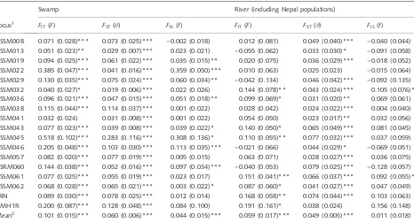
Separate analyses of the swamp and river buffaloF-statistics (Table 3) show significant differentiation (h) among the swamp populations for all loci, and among the river for most loci, with the mean over loci highly significant for both types. More loci show significant within-population inbreeding (f) for the swamp populations than for the river,
with the mean f over all loci not significant for the river populations. Pairwise estimates ofFST(Table S3) emphasize
the extent of population differentiation, with only 33 non-significant out of 561 tests. Differentiation among the Chinese swamp populations (mean FST= 0.024 ± 0.017)
was much less than among the SE Asian (0.165 ± 0.100). Within China, differentiation is primarily due to the DH population: the mean FST for DH vs. the other Chinese
populations (0.061 ± 0.010) is significantly greater (P< 0.001) than the meanFSTamong those other
popu-lations (0.019 ± 0.010). The Chinese river buffalo popula-tions (NL and MR) are significantly different from the Malaysian (UPM-M), Sri Lankan (SL-M and SL-S) and Nepal river populations. The Nepal wild population is significantly different from all the river populations (including the Murrah-type Nepal domestic), except the Nepal hybrid. Although the Nepal wild is phenotypically swamp type (like the Sri Lanka south population), the pairwiseFSTwith the
swamp populations are much larger; genetically the Nepal wild is like the river type.
The dendrogram (Fig. 2) again indicates the clear sepa-ration of the swamp and river populations, and of the Nepal wild among the river populations. Relationships among the swamp populations are unexpected, with the SE Asian populations separated into two groups by the Chinese
pop-Table 3F-statistics analyses, with significance determined by permutation tests in theFSTATprogram. Locus information is available on GenBank; for information about CSRM060, CSSM061 and CSSM062, see Mooreet al.(1995).
Locus1
Swamp River (including Nepal populations)
FIT(F) FST(h) FIS(f) FIT(F) FST(h) FIS(f)
CSSM008 0.071 (0.028)*** 0.073 (0.025)*** )0.002 (0.018) 0.012 (0.081) 0.049 (0.040)*** )0.040 (0.044) CSSM013 0.051 (0.023)** 0.029 (0.007)*** 0.023 (0.021) )0.055 (0.062) 0.033 (0.030)* )0.091 (0.058) CSSM019 0.094 (0.025)*** 0.061 (0.022)*** 0.035 (0.015)** 0.020 (0.075) 0.036 (0.029)*** )0.018 (0.052) CSSM022 0.385 (0.047)*** 0.041 (0.016)*** 0.359 (0.050)*** 0.010 (0.063) 0.025 (0.023) )0.015 (0.064) CSSM029 0.130 (0.035)*** 0.075 (0.024)*** 0.060 (0.034)** )0.042 (0.134) 0.046 (0.042)*** )0.092 (0.135) CSSM032 0.040 (0.027)* 0.019 (0.006)*** 0.022 (0.026) 0.144 (0.078)** 0.043 (0.024)*** 0.105 (0.076)* CSSM036 0.096 (0.021)*** 0.047 (0.015)*** 0.051 (0.018)** 0.099 (0.069)* 0.031 (0.020)** 0.069 (0.061) CSSM038 0.115 (0.044)*** 0.114 (0.037)*** 0.001 (0.022) 0.028 (0.042) 0.024 (0.022)*** 0.004 (0.040) CSSM041 0.032 (0.024) 0.031 (0.008)*** 0.001 (0.022) 0.054 (0.050) 0.023 (0.017)** 0.032 (0.056) CSSM043 0.077 (0.023)*** 0.039 (0.008)*** 0.039 (0.022)* 0.140 (0.050)* 0.065 (0.049)*** 0.081 (0.045) CSSM045 0.518 (0.102)*** 0.283 (0.116)*** 0.308 (0.136)* 0.110 (0.055)** 0.077 (0.032)*** 0.037 (0.059) CSSM046 0.205 (0.048)*** 0.103 (0.030)*** 0.113 (0.035)*** )0.021 (0.066) 0.044 (0.029)* )0.069 (0.051) CSSM057 0.082 (0.020)*** 0.077 (0.019)*** 0.005 (0.015) 0.063 (0.071) 0.028 (0.027)*** 0.036 (0.075) CSRM060 0.144 (0.038)*** 0.052 (0.016)*** 0.097 (0.034)*** )0.040 (0.053) 0.079 (0.025)*** )0.128 (0.057) CSSM061 0.077 (0.025)*** 0.055 (0.019)*** 0.023 (0.017) 0.151 (0.041)*** 0.066 (0.037)*** 0.092 (0.055)* CSSM062 0.068 (0.028)*** 0.065 (0.021)*** 0.003 (0.022)* 0.087 (0.060)* 0.041 (0.027)*** 0.047 (0.049) BRN 0.089 (0.030)*** 0.078 (0.025)*** 0.012 (0.014) 0.168 (0.058)** 0.074 (0.044)*** 0.103 (0.063) HMH1R 0.200 (0.087)*** 0.128 (0.048)*** 0.084 (0.100) 0.191 (0.161)* 0.038 (0.024) 0.156 (0.148) Mean2 0.101 (0.015)*** 0.060 (0.006)*** 0.044 (0.015)*** 0.059 (0.017)*** 0.049 (0.005)*** 0.011 (0.018)
These statistics are defined (Weir & Cockerham 1984) as the correlations between pairs of alleles: (i) within individuals (F); (ii) between individuals in the same population (h); and (iii) within individuals within one population (f). These are analogous to WrightÕs (1951)FIT,FSTandFIS.
*P< 0.05, **P< 0.01, ***P< 0.001.
ulations (except DH); Musuan, Sabah and Sarawak are most closely related to the eastern Chinese populations (FA and XF), and the remaining SE Asian populations are most closely related to the south-western (XL, DD and DC). Among the Chinese populations, DH is an outlier, nearest to the river populations. Network analysis (not shown) did not add further to interpretation of population relationships.
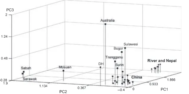
The PCA (Fig. 3) complements these population rela-tionships, with the swamp and river populations distin-guished by PC1. The Chinese populations (except DH) are tightly clustered; Musuan, Sabah and Sarawak are distin-guished from all the other swamp populations by PC2; and the other SE Asian swamp populations are separated from the Chinese by PC3.
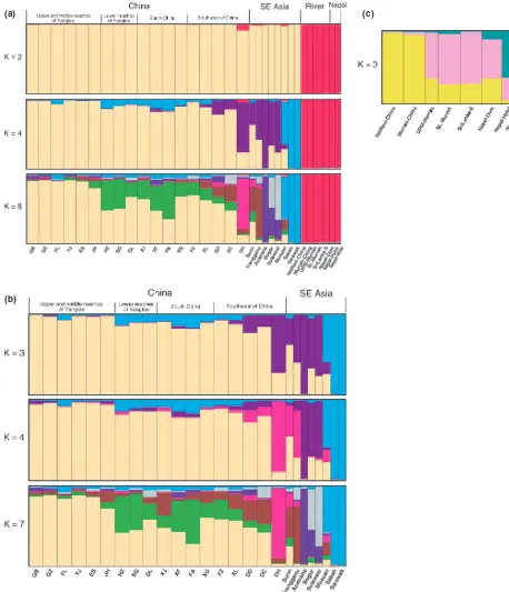
Structure analysis atK= 2 (Fig. 4) completely separated the river and swamp buffalo populations. The meanQ
val-ues (estimated membership of each cluster) were
0.993 ± 0.017 for the swamp populations in cluster 1 and 0.996 ± 0.004 for the river populations (including animals from Nepal) in cluster 2. The Chinese DH swamp population had the lowest Qvalue (0.917) among the swamp popu-lations, and Nepal wild had the lowest Q value (0.988) among the river populations. Given this very distinct sepa-ration of the two buffalo types, furtherSTRUCTUREanalyses
might have been restricted only to within each type (Coulon
et al.2008). This was done, but we also investigated higher
values of Kfor the full set of 34 populations, because of special interest in the two slightly outlying populations, Dehong and Nepal wild. The maximum Ln P(D) was observed forK= 12, but the plot first plateaued at K= 8, and the Evannoet al.(2005) method (hereafter referred to as the Evanno method) gave maximumDKatK= 4. The average inferred membership coefficients (Q) for each pop-ulation are shown forK= 4 andK= 8 (Fig. 4a). ForK= 4, the Chinese populations (except DH) are primarily cluster 1 (Q> 0.826), and the SE Asian populations (except Aus-tralia, Sabah and Sarawak) also have substantial coeffi-cients in cluster 1 (Q range = 0.235–0.636). The river
buffalo (including Nepalese animals) form a distinct cluster, with Nepal wild including a small component (Q= 0.016) in cluster 1. DH groups primarily with some of the SE Asian populations and has a small component from river buffalo. Musuan, Sabah and Sarawak comprise cluster 4, while the Chinese eastern populations have a small component in this cluster. For K= 8, DH is distinct from the other Chinese populations, which are represented in three main clusters. The SE Asian populations (except Sabah and Sarawak) are represented in more clusters than forK= 4, and the river buffalo (including Nepal) remain as a distinct cluster.
STRUCTUREanalysis of the swamp buffalo populations did
not give unequivocal results. The plot of Ln P(D) plateaued for K= 6–7, but then increased to K= 9, which had the maximum Ln P(D). However, the Evanno method gave maximum DK (36.30) at K= 3 and a slightly lower DK
(29.29) atK= 4. Inferred membership coefficients for each population are shown for K= 3, 4 and 7 (Fig. 4b). For
K= 3, cluster 1 comprises the Chinese populations (except DH), and Surin has a major component (Q= 0.623) in this cluster. Musuan, Sabah and Sarawak comprise cluster 2, and DH and the other SE Asian populations comprise cluster 3. AtK= 4, the major change is that cluster 3 above sep-arates into (i) DH, Surin and Trengganu, and (ii) Australia, Bogor and Sulawesi. AtK= 7, the patterns for DH and the SE Asian populations remain much the same, but the Chi-nese populations separate into three major groups, as found previously by Zhanget al.(2007). The overall patterns here are essentially the same as for the swamp at K= 8 in Fig. 4a.
When the river buffalo populations were analysed sepa-rately, the maximum Ln P(D) was at K= 4, but the plot plateaued at K= 3, and the Evanno method also gave maximumDKatK= 3. The average inferred membership coefficients are shown in Fig. 4c for K= 3, where the pri-mary cluster memberships are: (i) the two Chinese popula-tions, (ii) the SE Asian populations and Nepal domestic, and (iii) Nepal wild and hybrid.
Selection and population relationships
Three loci were identified as being potentially under selec-tion, with directional selection acting at CSSM045 (P< 0.01), and balancing selection acting at CSSM008 and
CSSM061 (bothP< 0.05). However, any selection had no significant effect on population relationships, as the phy-logeny, PCA and STRUCTURE results were essentially
un-changed when these three loci were deleted from the data set.
(a)
(b)
(c)
Discussion
Genotype identification for many microsatellite loci may vary among laboratories, so that the merging of indepen-dent data sets can be problematic. Presson et al. (2006, 2008) pointed out that merging is not necessarily a simple process of matching alleles one to one, and provided methodology and software to enable correct merging of data sets. Although our primary genotyping was performed in three different laboratories, comparison of allele frequency distributions and genotyping of a representative sample in two of the laboratories allowed us to readily and accurately combine our data sets for 18 of 20 loci. Consequently, we have genotype data for a reasonable number of microsat-ellite loci for 26 swamp buffalo populations that broadly cover its entire geographical distribution, as well as data for six populations of river buffalo, and for a small sample of the putative wild buffalo (B. arnee) and its hybrids with Murrah-type river buffalo. The river populations that we have sampled (except for SL-South and Nepal domestic) are descendants of animals imported from India and Pakistan, and their genetic variability may not truly represent that of the endemic breeds. Expected heterozygosities in our Mur-rah populations are less than those reported for this breed in India by Kumaret al.(2006, 0.78) and by Vijhet al.(2008, 0.69). Founder effects are most likely, as indicated by the numbers of animals imported for the two river breeds in China (Nili Ravi: ten males, 15 females imported from Pakistan in 1974; Murrah: three males, 32 females from India in 1957). Subsequent importations of frozen semen of both breeds in 1993 and 1995 probably contributed little to the adult animals we sampled in 2003. Nevertheless, all the river populations are clearly distinct from the swamp pop-ulations (Figs 2 and 3), although two of the swamp popu-lations (Musuan and DH) show evidence of introgression from river buffalo.
Murrah breed river buffalo were first imported into the Philippines in 1917 (Villegas 1958). As our Musuan sam-pled animals were all phenotypically swamp type, Barker
et al.(1997a), using allozyme data, considered introgression
unlikely. However, using microsatellites, Barker et al.
(1997b) showed that five of the sampled animals must have some cross-bred ancestry, and this introgression into the swamp population is well supported by theSTRUCTURE
anal-ysis (Fig. 4).
Zhanget al.(2007) showed the Dehong (DH) population to be quite distinct from other Chinese swamp populations, postulating that river buffalo ancestry had been introgres-sed by cross-breeding with river animals introduced from Burma (Myanmar). This postulate is apparently confirmed here, as one allele at each of six loci (CSSM029, CSSM038, CSSM046, CSSM057, CSSM061, CSSM062) otherwise found only in river buffalo (and three of them in Musuan) was observed at low frequency in DH. Recently, however, a river buffalo population from Tengchong county, Yunnan
Province (133 km by road from the DH locality) has been described, and local records show that 1029 river buffalo were imported from Burma and India in 1902 (Qu et al.
2008). While 30 animals were confirmed as having river karyotype (2n= 50), morphological criteria (colour pat-terns, horn shape) indicate introgression from swamp-type animals (Quet al.2008). The Nepal wild animals (putative
B. arnee) also carried five of the six river-specific alleles and
are phenotypically swamp type, so that there could have been past introgression from wild B. arnee into these far south-west China populations. That is, the swamp-type DH population has gained specific alleles, while the river-type Tengchong has gained some swamp-river-type phenotypic characteristics.
In historical times,B. arneeranged across a large part of India and east into mainland south-east Asia and south China (Cockrill 1984). Remnant populations are thought now to occur at various sites including southern Nepal, southern Bhutan, western Thailand, eastern Cambodia, northern Myanmar and at several sites in India (Hedges
et al. 2008). Archaeological, anatomical and historical
evidence supports the contention that both river and swamp domestic buffalo (Bubalus bubalis) are descended from
B. arnee(Cockrill 1984), and genetic evidence clearly points
to independent domestications of the two types (Lau et al.
1998; Kumar et al. 2007a; Lei et al. 2007; Yindee et al.
2010). The time of divergence of the river and swamp types has been estimated in various studies as from at least 10 000 years ago to 1.7 Myrs ago, but most probably about 128 000–270 000 years ago (see Kumar et al. 2007a), although even given this uncertainty, divergence occurred well before domestication.
Cockrill (1981) suggested that the river buffalo was domesticated about 4000–5000 years ago in the Indus valley, and possibly in the Tigris and Euphrates valleys, but from an analysis of mitochondrial D-loop variation in eight breeds of Indian river buffalo, Kumar et al. (2007b) con-cluded that the western region of the Indian subcontinent is the most likely area of domestication. In contrast, the time and place of domestication of the swamp type is very uncertain and is still subject to debate. Cockrill (1981) suggested that the swamp buffalo was domesticated in the Yangtze valley, also about 4000–5000 years ago. Chen & Li (1989) proposed an earlier time of 7000 years ago, but also pinpointed the area of domestication as the Yangtze valley. However, Epstein (1969), noting that domesticated buffalo were present in China by the time of the Shang dynasty (ca. 1766–1123 B.C.), suggested that domestic buffalo were introduced to China from south-east Asia prior to the Shang dynasty. He concluded that domestication of the indigenous
B. arneehad taken place at many locations, including south
and central China. However, there is no evidence that the endemic distribution ofB. arneeincluded central China. Liu
et al.(2006) concluded that archaeological study of Chinese
that domestic buffalo were most likely introduced from South Asia around the first millennium BC. Yang et al.
(2008), using D-loop mtDNA sequences, found no direct links between domesticated buffalo (B. bubalis) and the indigenous (but now extinct)B. mephistophelesfrom ancient China, again suggesting that the swamp buffalo was not first domesticated in China.
A consistent finding in studies of domestic animals with all molecular markers is that genetic variability decreases with increasing geographical distance from the centre of domestication (Groeneveld et al. 2010). As our sampled populations cover the broad distribution of the swamp type, can patterns of variation among them point to the likely region of domestication? PCA of the Chinese swamp popu-lations (excluding DH; Zhanget al.2007) showed gradients in allele frequencies from south to north (PC1) and from west to east (PC2). For both geographical gradients, Heand
allelic richness decrease, but regression coefficients are not significant. Although there are no significant differences in variability among the four clusters of the Chinese swamp populations (Fig. 4b), genetic variability (both Heand allelic
richness) significantly decreases from south-west to north-east along the southern transect (populations DD, XL, FZ, XF, XJ and FA – see Fig. 1): regression coefficients are
)0.0061 ± 0.0018, P< 0.05, and )0.0530 ± 0.0147,
P< 0.05, respectively. Among the swamp populations, genetic variability (both Heand allelic richness) is highest
for DH (possibly inflated by some river/wild ancestry) and Surin (Table 2), with Trengganu, DC, XL and DD showing next highest variability for one or other criterion. In a
dendrogram including only swamp populations (not
shown), DH clusters with Surin and Trengganu, while in the STRUCTURE analysis of the swamp populations (Fig. 4b,
K= 4), the membership coefficients are 0.883, 0.395 and 0.571 for DH, Surin and Trengganu, respectively. Even higher variability (He= 0.637–0.677 over all populations,
and He= 0.607 for the seven loci in common with ours)
has been recorded (Berthoulyet al.2010) for populations in the northern Vietnam province of Ha Giang, geographically close to the DD locality in China. Genetic variability also decreases from Surin south through Trengganu to Bogor and Sulawesi. Together, these results point to the domesti-cation centre for swamp buffalo in a region encompassing the far south of China, and northern Thailand and Indo-china. Archaeological findings support this conclusion. Groves (2006) noted that Ôthe oldest putative domestic buffaloes come from Neolithic sites in southern ChinaÕ, while Epstein (1969) stated that in north-east Thailand, buffalo bones first appear in archaeological sites about 1600 B.C., about the same time as wet rice cultivation. However, he assumed domestication in the Yangtze valley and thus considered that these facts indicated the introduction of domestic buffalo from somewhere else.
Sabah, Sarawak and Australia show the lowest levels of genetic variability. The Australian population is known to
have been bottlenecked at introduction into the country in the 1800s (Barker et al.1997a). As Sabah, Sarawak and Musuan are most closely related to the Chinese eastern populations (FA and XF – Fig. 2, Fig. 4a, K= 4; Fig. 4b,
K= 3), movement of animals from these eastern popula-tions through Taiwan to the Philippines and on to Borneo would place Sabah and Sarawak most distant from the apparent domestication centre. The genetic variability of the Musuan population would appear not to fit this scenario, but it is likely to have been inflated by the introgression of river buffalo noted earlier.
Given our postulated domestication centre for the swamp buffalo, our previous hypothesis (Lau et al. 1998) for the origin, demography and spread of domesticated buffalo needs to be revised as follows: (i) the speciesB. arneeevolved in mainland south/south-east Asia, with a range from the Indian subcontinent east to southern China; (ii) At some time in south-east Asia, the 4/9 translocation occurred to give the 2n= 48 swamp type; (iii) In the Indian subconti-nent,B. arneewas domesticated and evolved to become the various breeds of the river type; (iv) Following domestica-tion of the swamp type in the region encompassing the far south of China and northern Thailand and Indochina, and as indicated by the clear separation of the SE Asian popu-lations into two groups (Fig. 2), it spread south through peninsular Malaysia to the islands of Indonesia (Sumatra, Java and Sulawesi), north/north-east into central China, and then through an eastern island route via Taiwan to the Philippines and Borneo.
Acknowledgements
We thank Jacques Flamand for the organization and collection of the Nepal samples, and Hong Duong and Andrea Daley for assistance with genotyping the additional loci for these samples. This work was partially supported
by National Natural Scientific Foundation of China
(30901015), International S&T Cooperation Program (2008DFA31120), and the Fund for Modern Agro-industry Technology Research System.
References
Barker J.S.F., Tan S.G., Selvaraj O.S. & Mukherjee T.K. (1997a) Genetic variation within and relationships among populations of Asian water buffalo (Bubalus bubalis).Animal Genetics28,1– 13.
Barker J.S.F., Moore S.S., Hetzel D.J.S., Evans D., Tan S.G. & Byrne K. (1997b) Genetic diversity of Asian water buffalo (Bubalus bu-balis): microsatellite variation and a comparison with protein-coding loci.Animal Genetics28,103–15.
Chen Y.C. & Li X.H. (1989) New evidence on the origin and domestication of the Chinese swamp buffalo (Bubalus bubalis). Buffalo Journal1,51–5.
Cockrill W.R. (Ed.) (1974)The Husbandry and Health of the Domestic Buffalo. FAO, Rome.
Cockrill W.R. (1981) The water buffalo: a review.British Veterinary Journal137,8–16.
Cockrill W.R. (1984) Water buffalo. In:Evolution of Domesticated Animals(Ed. by I.L. Mason), pp. 52–63. Longman, London. Coulon A., Fitzpatrick J.W., Bowman R., Stith B.M., Makarewich
C.A., Stenzler L.M. & Lovette I.J. (2008) Congruent population structure inferred from dispersal behaviour and intensive genetic surveys of the threatened Florida scrub-jay (Aphelocoma cœrules-cens).Molecular Ecology17,1685–701.
Epstein H. (1969)Domestic Animals of China. Africana Publishing Corporation, New York.
Evanno G., Regnaut S. & Goudet J. (2005) Detecting the number of clusters of individuals using the software STRUCTURE: a simu-lation study.Molecular Ecology14,2611–20.
Excoffier L., Hofer T. & Foll M. (2009) Detecting loci under selection in a hierarchically structured population.Heredity103,285–98. FAO (2000)World Watch List for domestic animal diversity, 3rd edn
(Ed. by B.D. Scherf). FAO, Rome.
Flamand J.R.B., Vankan D., Gairhe K.P., Duong H. & Barker J.S.F. (2003) Genetic identification of wild Asian water buffalo in Nepal.Animal Conservation6,265–70.
Goudet J. (1999) PCAGEN, a program to perform a Principal Component Analysis (PCA) on genetic data (version 1.2). Available at: http://www2.unil.ch/popgen/softwares/pcagen. htm
Goudet J. (2001) FSTAT, a program to estimate and test gene diversities and fixation indices (version 2.9.3). Available at: http://www2.unil.ch/popgen/softwares/fstat.htm
Groeneveld L.F., Lenstra J.A., Eding H.et al.(2010) Genetic diver-sity in farm animals – a review.Animal Genetics41(Suppl. 1), 6–31.
Groves C.P. (2006) Domesticated and commensal mammals of Austronesia and their histories. In:The Austronesians Historical and Comparative Perspectives(Ed. by P. Bellwood, J.J. Fox & D. Tryon), pp. 161–73. ANU EPress, Canberra.
Hedges S., Sagar Baral H., Timmins R.J. & Duckworth J.W. (2008) Bubalus arnee. In: IUCN 2008. 2008 IUCN Red List of Threatened Species. http://www.iucnredlist.org
Hochberg Y. (1988) A sharper Bonferroni procedure for multiple tests of significance.Biometrika75,800–2.
Hubisz M.J., Falush D., Stephens M. & Pritchard J.K. (2009) Infer-ring weak population structure with the assistance of sample group information.Molecular Ecology Resources9,1322–32. Huson D.H. (1998) SplitsTree: a program for analyzing and
visu-alizing evolutionary data.Bioinformatics14,68–73.
Kaeuffer R., Re´ale D., Coltman D.W. & Pontier D. (2007) Detecting population structure using STRUCTURE software: effect of back-ground linkage disequilibrium.Heredity99,374–80.
Kumar S., Gupta J., Kumar N., Dikshit K., Navani N., Jain P. & Nagarajan M. (2006) Genetic variation and relationships among eight Indian riverine buffalo breeds.Molecular Ecology15,593– 600.
Kumar S., Nagarajan M., Sandhu J.S., Kumar N. & Behl V. (2007a) Mitochondrial DNA analyses of Indian water buffalo support a
distinct genetic origin of river and swamp buffalo.Animal Genetics 38,227–32.
Kumar S., Nagarajan M., Sandhu J.S., Kumar N., Behl V. & Nish-anth G. (2007b) Phylogeography and domestication of Indian river buffalo.BMC Evolutionary Biology7,186.
Lau C.H., Drinkwater R.D., Yusoff K., Tan S.G., Hetzel D.J.S. & Barker J.S.F. (1998) Genetic diversity of Asian water buffalo (Bubalus bubalis): mitochondrial DNA D-loop and cytochrome b sequence variation.Animal Genetics29,253–64.
Lei C.Z., Zhang W., Chen H. et al.(2007) Independent maternal origin of Chinese swamp buffalo (Bubalus bubalis).Animal Genetics 38,97–102.
Lessios H.A. (1992) Testing electrophoretic data for agreement with Hardy–Weinberg expectations.Marine Biology112,517–23. Liu L., Yang D. & Chen X. (2006) On the origin of the Bubalus
bubalisin China.Kaogu Xuebao2,141–78. [In Chinese]. Moore S.S., Evans D., Byrne K., Barker J.S.F., Tan S.G., Vankan D. &
Hetzel D.J.S. (1995) A set of polymorphic DNA microsatellites useful in swamp and river buffalo (Bubalus bubalis). Animal Genetics26,355–9.
Nei M. (1973) Analysis of gene diversity in subdivided populations. Proceedings of the National Academy of Sciences of the USA 70, 3321–3.
Nei M. (1978) Estimation of average heterozygosity and genetic distance from a small number of individuals.Genetics89,583– 90.
Nei M., Tajima F. & Tateno Y. (1983) Accuracy of estimated phy-logenetic trees from molecular data II. Gene frequency data. Journal of Molecular Evolution19,153–70.
NRC (1981)The Water Buffalo: New Prospects for an Underutilized Animal. National Academy Press, Washington, D.C.
Ota T. (1993)DISPAN: Genetic Distance and Phylogenetic Analysis. Pennsylvania State University, University Park, PA, USA. Piry S., Alapetite A., Cornuet J.M., Paetkau D., Baudouin L. &
Estoup A. (2004) GENECLASS2: a software for genetic assign-ment and first-generation migrant detection.Journal of Heredity 95,536–9.
Presson A.P., Sobel E., Lange K. & Papp J.C. (2006) Merging microsatellite data. Journal of Computational Biology13,1131– 47.
Presson A.P., Sobel E.M., Pajukanta P., Plaisier C., Weeks D.E., A˚ berg K. & Papp J.C. (2008) Merging microsatellite data: en-hanced methodology and software to combine genotype data for linkage and association analysis.BMC Bioinformatics9,317. Pritchard J.K., Stephens M. & Donnelly P. (2000) Inference of
population structure using multilocus genotype data. Genetics 155,945–59.
Pritchard J.K., Wen X. & Falush D. (2009) Documentation for structure software: Version 2.3. http://pritch.bsd.uchicago.edu/ structure.html
Qu Z., Li D., Miao Y., Shen X., Yin Y. & Ai Y. (2008) A survey on the genetic resource of Binlangjiang water buffalo. Journal of Yunnan Agricultural University23,265–9. [In Chinese]. Raymond M. & Rousset F. (1995) GENEPOP (version-1.2):
popu-lation genetics software for exact tests and ecumenicism.Journal of Heredity86,248–9.
Saitou N. & Nei M. (1987) The neighbour-joining method: a new method for reconstructing phylogenetic trees.Molecular Biology and Evolution4,406–25.
Schug M.D., Smith S.G., Tozier-Pearce A. & McEvey S.F. (2007) The genetic structure ofDrosophila ananassaepopulations from Asia, Australia and Samoa.Genetics175,1429–40.
Sokal R.R. & Rohlf F.J. (1981)Biometry. W. H. Freeman & Co., San Francisco.
Takezaki N., Nei M. & Tamura K. (2010) POPTREE2: software for constructing population trees from allele frequency data and computing other population statistics with Windows interface. Molecular Biology and Evolution27,747–52.
Vijh R.K., Tantia M.S., Mishra B. & Kumar S.T.B. (2008) Genetic relationship and diversity analysis of Indian water buffalo ( Bu-balus bubalis).Journal of Animal Science86,1495–502.
Villegas V. (1958) The Indian buffalo.Philippine Journal of Animal Industry19,85–90.
Weir B.S. & Cockerham C.C. (1984) Estimating F-statistics for the analysis of population structure.Evolution38,1358–70. Yang D.Y., Liu L., Chen X. & Speller C.F. (2008) Wild or
domesti-cated: DNA analysis of ancient water buffalo remains from north China.Journal of Archaeological Science35,2778–85.
Yindee M., Vlamings B.H., Wajjwalku W.et al.(2010) Y-chromo-somal variation confirms independent domestications of swamp and river buffalo.Animal Genetics41,433–5.
Zaykin D.V., Pudovkin A. & Weir B.S. (2008) Correlation-based inference for linkage disequilibrium with multiple alleles.Genetics 180,533–45.
Zhang Y., Sun D., Yu Y. & Zhang Y. (2007) Genetic diversity and differentiation of Chinese domestic buffalo based on 30 micro-satellite markers.Animal Genetics38,569–75.
Supporting information
Additional supporting information may be found in the online version of this article.
Table S1 Genotype data for all animals sampled in China, south-east Asia and Nepal, assayed for 18 microsatellite loci.
Table S2Allelic frequencies for each locus in each popula-tion.
Table S3Pairwise Fst among all 34 populations.