Dynamic Competition, Valuation, and Merger
Activity
MATTHEW SPIEGEL and HEATHER TOOKES∗
ABSTRACT
We model the interactions between product market competition and investment valu-ation within a dynamic oligopoly. To our knowledge, the model is the first continuous-time corporate finance model in a multiple firm setting with heterogeneous products. The model is tractable and amenable to estimation. We use it to relate current in-dustry characteristics with firm value and financial decisions. Unlike most corporate finance models, it produces predictions regarding parameter magnitudes as well their signs. Estimates of the model’s parameters indicate strong linkages between model-implied and actual values. The paper uses the estimated parameters to predict rivals’ returns near merger announcements.
INTUITION AND FUNDAMENTAL MICROECONOMIC theory tell us that product mar-ket dynamics should have a significant impact on valuation and financial in-centives. Yet, directly testable models relating these issues have been largely absent from the corporate finance literature. This paper helps fill some of these gaps by presenting a tractable framework for examining financial decision-making in a dynamic oligopoly with heterogeneous products. It shows that a firm’s competitive position can both profoundly influence its financial decisions and impact how the firm is influenced by the decisions of others. The model’s explicit closed-form solution allows one to estimate its parameters with ease. This paper takes advantage of this feature to apply the model to two financial questions: (1) cross-sectional valuation and (2) a horizontal merger’s impact on rival firms. While other directly testable dynamic models (those that pro-duce quantitative as well as qualitative forecasts) have been relatively rare in the corporate finance literature, notable exceptions include Leland (1994, 1998), Goldstein, Ju, and Leland (2001),Hennessy and Whited (2005, 2007),
Strebulaev (2007),Schaefer and Strebulaev (2008), andGorbenko and Strebu-laev (2010). However, to our knowledge, this paper is the first continuous-time corporate finance model that takes place in a multiple firm setting with het-erogeneous products. The oligopoly setting allows us to derive predictions re-garding the interaction between a firm’s competitive position and how both its own and its rivals’ decisions impact its immediate value and future responses.
∗Both authors are from the Yale School of Management. The authors thank Lauren Cohen, Engelbert Dockner, Alex Edmans, William Goetzmann, Alexander G ¨umbel, Jonathan Ingersoll, Uday Rajan, Raman Uppal, Ivo Welch, and seminar participants at the University of Toronto, UCSD, and the European Winter Finance Summit for their comments.
This paper analyzes a differential game based upon a variant of the
Lanchester (1916) “battle” model. In the model n firms compete for market share (share of industry sales) by spending funds to acquire each other’s cus-tomers. The model’s continuous-time setting allows for closed-form solutions that would be very difficult to obtain in discrete time. The model’s dynamic structure makes it straightforward to recover empirically unobservable pa-rameters such as consumer loyalty and firm-level spending effectiveness. Iden-tification in the model comes from market share evolution across firms and over time. Using accounting and financial data, one can use the model to generate estimates of these parameters and make predictions regarding the variation in firm values both within and across industries.
Although the model has several appealing features, its mathematical struc-ture, which describes competition for market share, may not apply to all in-dustries. However, it seems unlikely that any one model can properly describe every industry. The paper highlights the model’s empirical uses as well as limits by first presenting estimates of the ease with which firms can acquire market share. The set of industries, firms, and years for which this is accomplished is not exhaustive. For example, given that the model describes an oligopoly, industries with too many firms are excluded before attempting to generate es-timates. Nevertheless, they span a very broad array of 332 industries. While the model’s structure inhibits it from accurately describing every existing industry, this limitation also opens up a way to see if the estimated parameters reflect actual economic forces or something else. This is done by comparing how the model’s forecasts perform across industries where it should fit (mature indus-tries) with those where it should not (high growth indusindus-tries). Our tests verify that, relative to mature industries, the model’s empirical estimates for high growth industries are less accurate when it comes to valuing the underlying firms relative to mature ones.
each competitor. In this way, the paper is related to the substantial empirical literature documenting intraindustry spillover effects near corporate events, including: initial public offerings (Hsu, Reed, and Rocholl (2010)); mergers and acquisitions (Eckbo (1983, 1992),Fee and Thomas (2004), andShahrur (2005)); dividend announcements (Laux, Starks, and Yoon (1998)); bankruptcies (Lang and Stulz (1992)); corporate security offerings (Szewczyk (1992)); and cash policy (Fresard (2010)). The advantage of the model in this paper is that it pro-duces a testable structure for examining the cross-sectional variation in these spillover effects.
One important financial application of the model is that it can be used as a valuation tool for firms operating in oligopolistic product markets. As a starting point, we test whether model-implied firm values capture actual values for over 11,000 firm-year observations. This is done by taking parameters estimated with the model and then using them as inputs to the value functions derived in the paper. While market shares alone can only explain approximately 20% of the variation in firm values, the model explains over 43%. The fit of the model is driven by estimates of unobservable parameters such as industry-level consumer responsiveness, the company’s profitability, and the company’s ability to attract customers.
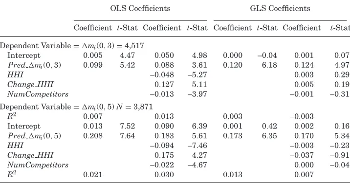
The model is also capable of generating forecasts of each firm’s eventual market share and how long it will take to reach it. We use the model to project 3- and 5-year-ahead changes in market shares and find correlations between actual and predicted changes in market shares of more than 0.08 and 0.15, respectively. These correlations are highly statistically significant. That the magnitudes of these correlations are substantially less than one suggests some of the limitations of the empirical implementation. However, as a benchmark, it is worth comparing the explanatory power of the model’s predicted changes in market share with other variables that have been used in the empirical corporate finance literature to describe the behavior of oligopolies (e.g.,Eckbo (1983)andShahrur (2005)). The three candidate variables that we examine are industry concentration (HHI), change inHHI, and the (log) number of firms in the industry. While these variables do offer additional explanatory power when added to the predictive market share regressions, the model-implied changes in market share remain statistically significant. Moreover, when we run a “horse race” among these variables using stepwise model selection based on the Schwarz Bayesian Information Criterion, we find that the model-implied changes in market share ranks highest of the four candidate variables. When a version of the model with stochastic market shares is applied to the empirical implementation, we find that the predictive power of the model is very robust. The market share prediction exercise in this paper is, to our knowledge, novel and may enhance current approaches to valuation.
The model’s flexibility allows it to be applied in many corporate finance settings.1 We present one example that revolves around a horizontal merger
1There is a literature on finance and product market interactions. However, most models focus
(M&A). In this setting, conflicting forces vie to determine the ultimate impact on rival firms. Rivals benefit from the reduced number of competitors. But they are hurt if the combined firm is a much stronger competitor than were the standalone firms. We take advantage of the structural model to disentangle these two effects. The model also shows how mergers between one pair of rivals can trigger profitable mergers among other pairs. This may prove useful in future research on how merger waves start.
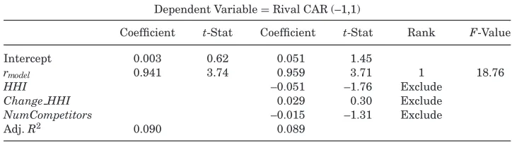
Estimates based on the M&A model indicate that it does help to explain the cross-sectional pattern of rival returns in response to a horizontal merger. Regressing actual merger announcement period returns against the model’s (out of sample) forecast yields parameter estimates showing that a 1% change in the model’s return is associated with about a 1% change in actual returns. TheR2statistics are also quite reasonable for an exercise of this type, coming
in at about 9%. Furthermore, this is accomplished by the model with the help of only two data series: revenues and cost of goods sold. By comparison, the purely empirical 11-variable model of customer and supplier returns in Fee and Thomas (2004)generates anR2 of 1.4% whileShahrur’s (2005) model of rival returns, with 10 explanatory variables, generates an R2 of 9%. These analyses fit observed returns using a variety of explanatory variables that are potentially correlated with returns. Here the exercise is forward-looking. Our forecasts are based on the estimated model parameters using only data that were available prior to the forecast date.
The model’s structure also allows one to decompose the effect of a merger on industry rivals in ways that are impossible with a static model as guidance. In particular, it can be used to estimate the gain from a reduction in the number of competitors versus the loss from facing a potentially stronger rival. Based on the empirical estimates, if within-industry mergers did nothing but soften competition through the reduction in the number of firms, then the median rival’s value in our data would increase by about 2.52%. Similarly, if the only effect was to generate a stronger competitor, the rivals would lose about 0.30% in value. This makes intuitive sense. Prior studies show that mergers create considerable value for the combining companies.Betton, Eckbo, and Thorburn (2008) report abnormal returns to the combined firm of more than 2%. Yet, studies going back toEckbo (1983, 1992) also show that rival returns are small. The model reconciles these results by providing estimates of the two competing forces. It also shows that nonlinearities may matter. On average, the model forecasts a rival return of 0.36%. (In actuality, firms in our database earn a mean return of about 0.61% and a median return of 0.47%.) This comes from a 2.22% gain due to the reduction in the number of firms in the industry, which is partially wiped out by a 1.86% reduction in rival firm value, caused by the reduction in the number of competitors along with a new stronger firm. This
offsetting effect occurs because the reduction in the number of competitors along with the creation of a stronger rival creates an interaction effect that works to the newly created firm’s relative advantage.
The paper is organized as follows. Section I presents the basic model, in-cluding the solution to the infinite horizon case. Section II presents results from estimating key parameters in the model. Section IIIpresents the M&A application.Section IVconcludes. Finally, the Appendix contains details on the derivation of the model’s equilibrium.
I. Basic Model
A. Players, Timing, Dynamics, and Strategies
TheLanchester (1916)battle model was originally designed to study military strategy. Since then variants have been widely used in the marketing literature to examine advertising strategies (see, for example, Erickson (1992, 1997),
Fruchter and Kalish (1997), Bass et al. (2005), Wang and Wu (2007); for a review, seeDockner et al. (2000)), although, to our knowledge, not in the form presented here. This paper’s adaptation creates a differential game in which competition among oligopolists selling heterogeneous goods can be explored.
Considern risk-neutral value-maximizing firms battling for market share. Let ui(t)≥0 represent the dollars spent by firm i on gaining market share at instant t. Let si denote the effectiveness of spending. Note that spending to acquire a competitor’s customers (ui) can imply a wide range of activities, including advertising, new product design, opening new stores, and R&D. The si parameters can represent the relative attractiveness of each firm’s product and/or the relative quality of its marketing campaigns.
The market share of firmiat timetis denoted bymi(t). Time is continuous and there is a finite starting point att=0. Given the initial conditionmi(0),mi evolves as follows:
dmi =
φ(1−mi)uisi−mi
j=iujsj
n
j=1ujsj
dt, (1)
Since this paper seeks to examine economic outcomes within industries that are natural oligopolies, an assumption about consumer behavior is needed. If the industry is characterized by positive network externalities then it is a nat-ural monopoly. In this case, once a firm’s market share reaches a tipping point, it eventually acquires all of the market. In a natural oligopoly such as the one described in this paper, however, that is not the case. Instead, it must be that every firm has some consumers that find its offerings exceptionally attrac-tive even if most people use a rival’s products. For example, McDonald’s is the largest fast food restaurant chain in the United States. Nevertheless, many con-sumers only eat at Burger King.Equation (1)’s structure captures this general property: firms produce heterogeneous products and consumers have heteroge-neous preferences. This formulation also implies that there are diseconomies of scale in spending to attract customers. Differentiating (1) shows that it is monotonically decreasing inui. Essentially, the first dollar a firm spends on its customer acquisition program does more to attract buyers than does the sec-ond, and so on. This is natural since customers that have a strong preference for a firm’s product line should be easy to bring in. As one moves further away in preference space, the firm is then forced to spend even more to acquire new customers. For example, Burger King’s loyal customers will probably continue to eat there, no matter how much McDonald’s spends to attract them. On the other hand, the converse is true too—there are fans of McDonald’s that Burger King cannot attract.
Related to the issue of ensuring that the model describes an oligopoly is the assumption that spending effectiveness and actual dollars spent are multiplica-tive. That is, the relative value of a dollar spent by any two firms is constant. Other formulations like a power relationship, for example, usi
i , would alter that. In this case, the relative value of each dollar spent would either increase (si > 1) or decrease (si < 0) with a firm’s own spending. In equilibrium, we suspect that, with si <1, the results would be qualitatively similar to what the current setting yields. But, of course, tractability would suffer. Forsi>1, however, as spending increases the firm would become even more effective in attracting consumers. In the end, this would produce an industry with what amount to network externalities and thus a natural monopoly.
The last element inequation (1) isφ. This is a consumer “stickiness” param-eter. High values imply that customers are easy to move in a short period of time from one firm’s product line to another’s. Low values imply the opposite. Thus, one imagines thatφhas a high value in the fast food industry since peo-ple purchase meals several times a day and purchases do not have to be made repeatedly from the same firm. Conversely, it is likely thatφis low in industries that sell heavy equipment such as backhoes. These are durable goods that are only replaced every few years. Furthermore, once a firm has committed itself to a product line, it may be costly to switch vendors if the products interact with each other.2
2Further intuition can be garnered by looking atφ’s extreme values. Setting it to zero implies
Before specifying the profit function, three additional observations from the formulation of dm (equation (1)) are worth noting. First, the discussion in the paper assumes ui ≥0 in equilibrium. However, the equations are solved unconstrained and in principle there exist exogenous parameter sets such that one would need to solve a constrained problem instead. Since this paper focuses on mature stable industries, where exit is of secondary importance, it is useful to restrict attention to cases in which the unconstrained equilibrium values of u are always strictly positive. Later, the sufficient exogenous parameter conditions needed to do this are laid out.
Second, dm is discontinuous whenever a firm “gives up” and sets its ui to zero. This is a result of the model’s assumption that it is relative spending that matters and ensures that the model is unit free. Beyond that, thedmequation’s behavior when a firm setsui =0 also generates a particularly useful statistic, which we call the industry half-life. That is, if a competitor sets ui equal to zero, one can estimate the length of time it takes that firm to lose half of its customers when the other firms continue to compete for them.3
Third, the law of motion shown in equation (1) differs from the market-ing literature, which typically examines a duopoly model with eitherdm/dt= u1(1−m)−u2mordm/dt=u1√1−m−u2√m(Dockner et al. (2000)). One
ad-vantage of usingequation (1) instead is that it is unit free. This eliminates the problem that changing the unit of currency also changes the rate at whichm changes over time. Another important advantage to this formulation is that rel-ative (rather than absolute) measures of spending are likely to be most relevant for within-industry dynamics.
Returning to the model, instantaneous profits are assumed to be proportional to market share and include a fixed operating cost. Letαi denote the revenue generating ability of firmiper unit of market share. Profitsπ equal revenues minus both spending on market share competition and a fixed operating costfi:
πi(t)=egt(αimi(t)−ui(t)− fi). (2)
The termgrepresents the industry’s rate of growth. It is assumed that, as the industry grows larger, profits and costs grow proportionately.4 Note that
spending by each firm does not impact the industry growth rate. Thus, the model should be thought of as applying to an industry in which innovations tend to change customer loyalties rather than increase overall demand. For example, an easier-to-swallow aspirin will probably cause consumers to switch
other end, asφgoes to infinity, customers instantly switch vendors and do so en masse at the drop of a coupon.
3Section I.C.1.bgoes into greater detail and contains examples highlighting the half-life
statis-tic’s implications whileSection I.C.1.acontains estimates of its value. If one dislikes the model’s behavior whenuiequals zero, adding a fixed constant toequation (1)’s denominator will eliminate
it. However, this comes at the cost of having a half-life without further assumptions.
4In general for a starting value ofπ(0) inequation (2), multiply each equality by that amount.
brands but seems unlikely to lead to an overall increase in pill consumption. One can modify the model to allowgto depend onuibut at the cost of a closed-form solution. We therefore leave g as an exogenous parameter making the model better suited for an analysis of lower growth industries, as in the aspirin example. Still, the model is quite flexible in its ability to describe differences across industries. If one thinks that it is easier to acquire market share in faster growing industries, this can be accommodated by simply setting φ to a larger value ifg is larger. In terms of the mathematics it does not matter if market share growth comes from taking in newly entering consumers or stealing existing ones from rivals.
The profit function in equation (2) is similar to that used in many applica-tions, for example, the standard Cournot oligopoly model. Because profits are linear in market share (sales), the firm’s production function exhibits constant variable costs. At the same time, the fixed operating cost (fi) implies that there are economies of scale. (Iffiequals zero then total production costs are simply proportional to sales. There is nothing in the model’s analysis that requires a strictly positive value offi.) For many, although not all, industries these seem like reasonable assumptions. For example, a fast food chain purchases raw materials (beef, potatoes, cleaning supplies, ovens, etc.) in a competitive envi-ronment. In cases like this, variable costs should be approximately proportional to sales.
To help streamline the exposition, details regarding the derivation of the model’s equilibrium conditions can be found in the Appendix. There we solve a general version of the model. The main text then employs the general solution to discuss various special cases. Thus, in the main body of the paper, equilibrium conditions are simply stated without proof except for occasional references back to the Appendix.
B. The Equilibrium Value Functions
Letrdenote the instantaneous discount rate. Assume that the discount rate exceeds the industry rate of growth (r>g). Defineδ =r−g. Firms chooseui to maximize expected discounted profits:
∞
0
(αimi(τ)−ui− fi)e−δτdτ. (3)
be written as5
Vi(m,t) = ai + bimi (4)
within the scenarios considered in this paper.6As shown in the Appendix,
ai =
φαi[αisiz−(n−1)]2 δ(φ+δ) (αisiz)2 −
fi
δ (5)
and
bi =
αi
φ+δ. (6)
Inequation (5) above,zequals
z=
n
j=1
1 αjsj
(7)
and can be thought of as a measure of the competitive strength of firms within an industry. Later on it will also be useful to define its mean as ¯z=z/n. Intu-itively, a firm is a strong competitor if it can both profit from gaining market share (αj) and economically attract customers (sj). Since the units of measure are arbitrary (dollars or euros forαand some measure of effective marketings) what matters isz, the ratio of one firm’s competitive strength relative to that of each rival. As a result, the termzappears repeatedly throughout the model’s solution.
C. Equilibrium
C.1. Spending on Customer Acquisition and Retention
In the Appendix, we show that V′
i has as its solution αi/(φ +δ). Using the definition ofzand some algebra, one can show that
ui=
αiφ(n−1)[αisiz−(n−1)]
(φ+δ)(αisiz)2 , (8)
which characterizes the equilibrium strategies that we seek. Observe that, if there are no fixed costs (fi=0), equilibrium spending remains unchanged. This is becauseV′
i is a function of onlyαi,φ, andδ.
5We focus on pure strategies here. However, given the intuition that mixed strategies might
allow firms to collude to limit wasteful spending, we examined a two-firm version of the model with this property. In it, one firm receives an unanticipated (privately observed) positive shock to its profitability. In that setting, there exists an equilibrium in which spending on market share acquisition does not increase to reflect the positive shock. In this equilibrium, both firms earn more than they would in a full information environment.
Since the focus of this paper is on an ongoing oligopoly, we need to assume the exogenous parameter values are such that no firm wishes to exit the indus-try. This naturally requires setting each firm’s fixed costs low enough that it is worth more if it operates than if it closes down. A sufficient condition to guar-antee this is to selectfismall enough that (5) is strictly positive. However, that will only hold in the steady state if firms actually compete for market share and sufficiently weak firms will not. So long as a firm’s spending on market share is strictly positive, the law of motion (1) guarantees a strictly positive market share along all possible paths. However, if spending (ui) is negative this need not be the case. Thus, in keeping with this paper’s focus, assume every firm is strong enough thatαisizi−(n−1)>0.7
From equation (8), one can examine how competitive forces impact equi-librium spending. It is straightforward to show that spending is strictly increasing in consumer responsiveness,φ. When there is a greater incentive to spend money to attract customers, firms do so. Spending is strictly decreasing in the discount rate net of industry growth (δ) since it lowers the present value of the revenue a new customer brings in. As one might expect, firms that earn a greater profit per sale (higherαi) spend more on customer acquisition because they are worth more to acquire. The derivative ∂ui/∂αi is positive as long as αisiz>2−2/n. As noted above, if every firm in the industry is competing for customers, then αisizi >n − 1 and for n ≥ 2 this implies that αisizi > 2 − 2/nas well. However, the impact of spending effectiveness (si) on equilibrium spending depends on a firm’s competitive strength. The derivative ∂ui/∂si is positive as long asαisiz>2(n−1). Thus, if the firm is strong enough, higher values ofsiwill lead to higherui, otherwiseuigoes down.8There are two forces at work here. One is the standard trade-off. Firms with higher values ofsican spend less and still attract customers. Weak firms find that the best option is to “split the difference” whensi increases by reducingui. For strong firms, the gain in market share from spending yet more on customer acquisition is just too strong to pass up for the offsetting gains a reduction inuiwould bring. But there is a second factor at play that only becomes apparent in a multiple-firm model. When firms are relatively weak, increases in spending are met with more aggressive spending by rivals, which decreases the incentives to spend more. This can be seen by an examination of ∂ui/∂(αj=isj=i), which is also positive as long asαisiz>2(n−1). Comparative statics usingequation (8) are summarized inTable I.
7Notice that asngoes to infinity the industry in this model becomes perfectly competitive. For
the inequality to hold in the limit, one needsαisiz¯>1 for each firmi. But this can only be true
if every “below average” firm is driven out, leaving a set of equally strong competitors. This, of course, conforms to the usual microeconomic view of what should happen in such industries.
8It is easy to generate examples in which there are firms in the industry for which the
compar-ative static goes both ways. Consider an industry with four firms. Three have values ofαisi=1
and one has a value equal to 2. In this casez=3.5. For the lowαisifirms,αisiz=3.5>3 so they
compete for market share, but sinceαisiz=3.5<6, for them∂ui/∂si<0. For the highαisifirm,
Table I
Change in the Equilibrium Spendingui fromEquation (8)
Derivative with
respect to Economic Interpretation Sign Condition
φ The impact of an increase in consumer responsiveness
increases spending to acquire customers. +
All firms
δ An increase in the discount rate reduces spending to acquire customers.
– All firms
αi The impact of an increase in firm profitability per unit
market share on spending to acquire customers. +
Large firms
si The impact of an increase in the attractiveness of a firm’s
products on spending to acquire customers.
+ Large firms
(αj=isj=i) The impact of an increase in the competitive strength of a
rival on spending to acquire customers.
+ Large firms
C.1.a. Entry and Exit: Impact on Customer Acquisition and Value
With the model’s solution and restrictions on the exogenous parame-ter values in place, one can now analyze the equilibrium responses to changes in ¯z, the competitive environment. Since the paper’s empirical sec-tion examines the impact of a merger between rival firms, it is useful to begin by seeing how a change in the number of competitors (n) alters equi-librium spending across firms. In a standard Cournot model, adding com-petitors decreases the equilibrium quantity produced by each firm. Firms “accommodate” the new entrant. Is the equivalent true here? Does adding a firm to the industry cause its competitors to reduce their spending on customer acquisition, with the incumbents all settling for smaller mar-ket shares? Because the model allows for heterogeneous firms this ques-tion cannot be answered until one first specifies what type of competitor is being added. A natural choice is to assume the new firm is “average” in that it leaves ¯zunchanged. Assuming this is the case, differentiating (8) leads to the following proposition.
PROPOSITION 1: Increasing n while holding z constant leads to the following¯ spending change by firm i:
dui
dn =
φ[nαisiz¯+2(1−n)]
n3(φ+δ)α
i(si¯z)2
. (9)
cross-derivative is ambiguous whereas for an average or below average com-petitor in the industry (i.e.,αisiz¯≤1) one can show it is strictly positive. Thus, if the model captures the competitive features of an industry, then looking across companies from weaker to stronger, the response to an increase innshould be increasing in the data.
Compare the result in Proposition 1 to its analog within a standard homoge-nous product Cournot model. In a Cournot model, entry induces every firm to accommodate the new firm by cutting back on production. Whether a firm is strong or weak, it scales back on the control variable. In this paper, this is generally false for very strong firms. Empirically, this dichotomy may look like “predatory behavior” on the part of an industry’s leaders as these are the firms most likely to have large values ofαi, si, and thusαisiz¯.
Based on the above results, intuitively one might now expect to find that very strong firms actually gain market share if a new firm of average competitive ability enters the market. However, it turns out that this is not true. To begin the analysis, the next proposition derives the steady state market share of each firm ( ¯mi) in terms of the model parameters.
PROPOSITION2: The steady state market share of each firm equals
¯
mi = 1−
n−1
αisin¯z
. (10)
Proof:Steady state occurs whenmiis such thatdmi/dt=0, or
mi =
uisi
n
j=1uisi
. (11)
To generate (10) substitute (8) into (11). For the denominator of (11) this pro-ducesn
j=1ujsj=1/z, after using z=nj=11/αisi. Some simple algebra then
yields (10). Q.E.D.
Two somewhat obvious empirical implications arise immediately from Propo-sition 2. The first is that in the steady state stronger competitors (those with higher values ofαisi) obtain a larger share of the market. Second, adding a new competitor of average competitive strength (thus leaving ¯zunchanged) reduces the market share of every firm.
A more interesting set of empirical predictions arises from a closer exami-nation of the model’s cross-sectional attributes. Proposition 1 shows that very strong competitors increase their spending on market share acquisition in re-sponse to entry. Proposition 2, however, demonstrates that in the end they still lose some customers. But the additional spending is not in vein. The increased spending by stronger firms causes them to lose fewer customers than their weaker rivals to the new entrant. Some minor algebra shows that the cross-derivative of a firm’s steady state market share to the number of competitors and its own competitive ability (∂2m¯
industry, weaker firms will lose a greater fraction of the market than stronger firms. This happens even though the weaker firms begin with smaller fractions of the market to begin with. Given their relative inability to compete effec-tively, their best response is to essentially cede market share and not fight to retain it.
C.1.b. Consumer Responsiveness and Corporate Values
Another variable impacting long-run industry values is the degree to which consumers respond to corporate entreaties (φ). Plugging ¯mi intoViyields firm i’s steady state value:
Vi( ¯mi) =
αi[αisiz−(n−1)][(φ+δ)(αisiz)−φ(n−1)] δ(φ+δ) (αisiz)2 −
fi
δ. (12)
Differentiating (12) with respect to the consumer responsiveness parameter shows that, in the steady state, firms are worth less if they are in an industry in which consumers are easily drawn away. The reason for this can be found in the equilibrium values ofuiand the fact that a firm’s steady state market share ( ¯mi) does not depend onφ. An examination of equilibrium spending to attract customers (equation (8)) shows that firms spend less if consumers become less responsive. Thus, every firm in an industry benefits fromφ’s reduction because they earn the same steady state revenue stream while wasting fewer resources trying to lure away each other’s customers.
The effect of consumer responsiveness on corporate policy as outlined above is easily seen in real industries. For example, if beer drinkers exhibited greater loyalty to particular brands, brewers would undoubtedly advertise less and collectively earn higher profits. From 1981 to 2008, per capita beer consump-tion in the United States fell from 24.6 to 21.7 gallons despite heavy product advertising (USDA, 2010). But no one brewer can reduce its own spending without losing customers to competitors. Thus, in equilibrium, they end up ad-vertising just to retain their current market shares even amid stagnant sales. Compare this to the situation in, for example, natural gas distribution where consumers are locked into a single supplier and thus these firms do relatively little advertising.
Additional economic intuition can be gained by looking at what can be called the industry “half-life.” This represents the time it would take a firm to lose half its customers if it stopped working to keep them by settinguito zero. This value can be calculated from (1) and turns out to equalh=ln(2)/φ.
equilibrium values ofuiinto (1) yields
dmi
dt =
φnαisi¯z−(n−1)
nαisi¯z −
φmi, (13)
which has a solution formi(t) of
mi(t) =
nαisiz¯−(n−1) nαisi¯z
(1−e−φt). (14)
Thus, the new entrant can be expected to capture a quarter of its steady state market share aftert=hyears. In this example, the incumbent firms’ reaction to the entrant cuts the entrant’s rate of growth in half.
Growing, newly public firms can be difficult to value, in part because of challenges associated with forecasting their future cash flows. Suppose the entrant in the above example goes public upon reaching a quarter of its steady state market share. Again solving the ODE one finds that the entrant’s growth decelerates from its pre-IPO levels. While the firm gained a quarter of its long-run market share in the firsthyears of its life, it will now take the same amount of time to go from one-quarter to three-eighths. What this means is that, if one can estimate the value of h associated with a particular industry and each firm’s s andα, the model can be used to make predictions about each firm’s long-run market share, profitability, and spending on customer acquisition. In addition, it offers predictions about the time it takes new entrants to reach particular market share levels. These estimates should also help predict cash flows and improve valuation in IPO studies.
C.2. Stochastic Market Shares
Prior to applying the model to real world data, it is useful to generalize the law of motion governing the change in market shares (equation (1)) to include a stochastic component. This allows one to expand the interpretation of the error term in empirical work from that of measurement error alone to one that also includes randomness in the underlying economy.
Each firm in an industry competes withn– 1 others. It therefore facesn– 1 stochastic processes relating where its customers may arrive from or depart to. Combined with the discussion above, the original law of motion describing firmi’s market share formulated inequation (1) becomes:
dmi =
Using (15), the instantaneous variance for each firm’s market share is σ2mi(1−mi) and its covariance with firm j is −σ2mimj. Overall then, the variance–covariance matrix governing the change in market share can be written as
While adding a stochastic term to equation (1) induces uncertainty in the value of each firm going forward, it does not change the solution to its opti-mization problem. The solution to the original deterministic problem involves a value function (V) that is linear in the state variablem. Thus, the second or-der term (∂2Vi/∂m2
i), which interacts with the variance–covariance matrix (16), equals zero in the Hamilton–Jacobi–Bellman (HJB) equation for the new opti-mization problem. This implies that the solution to the deterministic problem is also the solution to the problem with stochastic elements.9
Even though adding stochastic terms leaves the solution to the control prob-lem unchanged, it does add new eprob-lements to the model’s properties. With the addition of the Weiner processes, market shares no longer follow deterministic paths and thus neither do firm values. Combiningequations (4), (13), and (15) implies
Thus, the instantaneous variance inViis proportional to that ofmi.
II. Estimation
A. Outline
A primary goal in this paper is to incorporate market share dynamics re-sulting from product market competition into the analyses of firm valuation
9A more extensive discussion of this general property relating when the deterministic and
Table II
Possible Empirical Proxies for the Model’s Parameters
Parameter Description Possible Empirical Proxies
m Market share Share of total industry
Sales Assets
u Spending to gain market Advertising
share R&D
Capital expenditures Coupons
Loyalty programs φ,αsz Consumer responsiveness
and relative
competitive strength.
Estimation based onequation (1), using equilibrium spending given inequation (8) and equilibrium market shares inequation (10) to obtainφ, ¯mi, andαsz(seeequation
(19))
Estimation based on the discrete-time version ofequation (1) to obtainφand
mi,t+1−mi,t=φ
uisi(1−mi)−miNj=iujsj N
j=1ujsj
Estimation ofφ,α,andsbased onequation (4)
α Revenue-generating Operating profit
ability Estimation based onequation (2) or (4)
f Costs of operations (fixed) Operating expenses (net of proxy for market share spending)
Estimation based onequation (2) or (4)
δ r–g: discount rate minus Industry cost of capital industry growth rate Industry growth rate
Estimation based onequation (4) V Value of the firm Equity market capitalization+debt
and financial decision-making. One important advantage of the main model is that it is well suited for empirical analysis. AsTable IIshows, several readily available empirical proxies can be used. In this section, we take the first of the three possible approaches to the estimation ofφthat are suggested inTable II.
Equation (1) provides a mechanism through which the consumer responsive-ness parameterφcan be estimated for each industry. Substituting equilibrium values of spending fromequation (8) intoequation (1) and usingequation (11) to define steady state market share ( ¯mi) gives:
dm=φ( ¯mi−mi(t))dt, (18)
which has a solution formi(t) of:
mi(t)=m¯i+(mi(0)−m¯i)e−tφ. (19)
regardless of whether the stochastic term is included in thedmi equation. We rely onequation (19) to estimate bothφand ¯mi using nonlinear least squares. As described in more detail in Section I.B later, identification in the model comes from market share evolution across firms and over time.
Recall that φ captures consumer responsiveness, and is expected to be greater than zero. If consumers are unresponsive to spending, then they continue to purchase from their current firm no matter how much is spent to attract them. In estimation, the only restriction that we impose on φ is that it is nonnegative and less than 25 (in our annual estimation, 25 would correspond to a customer half-life of just 10 days, implying extreme disloyalty). This rarely binds in the data. Recall from Proposition 2 that ¯mi = 1−αni−sin1¯z. Thus, parameter estimates fromequation (19) also provide estimates of each firmi’s competitive strength,αisiz.
B. Identification
For each industry and year, we estimate the model using data from rolling 10-year intervals and assume that φ remains constant over each interval. Since there are N firms and market shares have to add to one, there are N – 1 independent observations in each period. To ensure that annual mar-ket shares do not add to one, we eliminate the j smallest firms (i.e., those with t = 0 market shares of less than 3%, or the smallest firm in the in-dustry if there are no firms with market shares of less than 3%). There are 10 years in the estimation window, and we therefore use 10(Nt – j) obser-vations to estimate the N – j+1 unknown parameters ( ¯mi for each of the n – j firms, plus φ). In reality, firms enter and exit industries, so there are actually 10(Nt – j) observations for each industry. Requiring t = 0 market shares that are greater than 3% reduces noise in parameter estimates due to small firms moving in and out of the sample (because we focus on larger firms that are in the sample at the beginning of the estimation window). Assuming φ remains constant over the sample period, we estimate the parameters in
equation (19) by minimizing the total sum of squared errors via nonlinear least squares.
Identification in the empirical estimation comes from changes in market share over time (to identify ¯mi) and across firms (to identifyφ). To illustrate how this is done, one can think of a two-step iterative process. The first step starts with initial valuesmi,0from the data and a starting guess for the industry
value ofφ(we use one in the estimation). We then plug these into (19) to produce a set of errors over time for each firmi. An initial estimate of ¯miis next produced by finding the value that minimizes the sum squares for firmi’s errors. This procedure is then repeated across all firms in the industry to produce an initial vector of ¯mi. Given a set of ¯mi, the second step finds the industry value of φ that minimizes the cross-sectional panel of squared errors in (19). Using the new φ as a starting value, this two-step process can be repeated until convergence is obtained forφand all of the ¯mi.In practice, the nonlinear least squares estimation of bothφ and them′
an iterative process (Gauss–Newton method) and given starting values for all unknown parameters.
Given the estimated steady state market shares (mi) and Proposition 2, the firm-specific variable αisiz comes directly from the estimation described above. One benefit of the model and our estimation approach is that we do not need to estimate the firm-specific parameters. This is because it is only a firm’s relative competitive strength (combinedαisiz) that impacts equilibrium spending and value.
C. Data and Parameter Estimates
C.1. Data and Sample Selection
The only data required to estimate φ and ¯mi are the market shares of all firms in the industry. Market share,mi,t, is defined as firmi’s sales divided by the sales of all U.S. headquartered CRSP/Compustat firms in the Compustat four-digit SIC code during year t.10 We choose four-digit codes to mimic the
model’s industry setting as closely as possible. Compustat codes are used due to findings in the literature (e.g.,Guenther and Rosman (1994)) that linkages among firms based on these codes are higher than with CRSP SIC codes.
The initial sample consists of all firms for which there is nonmissing infor-mation on annual sales and all four-digit SIC industries in which there are fewer than 20 firms. The oligopolistic structure described in the main model makes industries with a large number of firms inappropriate in the context of this paper. We also exclude all industries with fewer than two publicly traded firms during the entire sample period. As noted earlier, we estimate the model annually. Estimates for year t are obtained using rolling 10-year data inter-vals covering yearstthrough yeart+9. We restrict our attention to firms for which we have data for more than 5 of the 10 years of each estimation interval. The estimation period begins in 1980 and ends in 2004.11 Given the model’s
assumptions thatr>gand that there is no entry or exit, we exclude industries that are growing (or shrinking) at very high rates. To do so, we impose the filter r>|g|wheregis the average sales growth by all firms in the industry during the estimation window andris the expected rate of return on the stock market at the beginning of the estimation window.
The observations are pooled for each industry and then the industry- and firm-specific parameters φand αisiz, respectively, are estimated according to (19). For each 10-year rolling window, we also estimate firm-level parame-ters αi and fixed costfi based on OLS estimation of a modified equation (2): πi(t)=egt(αimi(t)−ui(t)− fi). Rather than use proxies such as advertising or
10The main model assumes no exit; however, due to changing product mix and SIC code
re-classification for some firms, we adjust for “exit” in the data by assuming that each firm in the industry gains market share from the exiting firm, in proportion to its current market share. We do not need to adjust for entry because data filtering requires that all firms be in the sample at the beginning of rolling intervalt.
11Data for estimation are from 1980 to 2009. Estimates end in 2004, given the data requirement
Table III
Summary of Estimated Parameter Values
This table presents summary statistics for the estimated parameter values for the 12,643 firm-year observations. Estimates for industryφand firm ¯miare based on nonlinear least squares estimation
ofequation (19), which is based on the law of motion for market sharedm.Firmi’s market share, mi(t), is defined as the share of sales of all CRSP/Compustat firms in the industry. The initial
sample consists of all four-digit SIC codes with fewer than 20 firms for the period 1980 through 2009. Estimates are obtained for firms with market shares greater than 3%. Industries withr <|g|are excluded from the estimates. The individual firm profitability parameters (αi) per unit
market share (millions of 2007 dollars per year) are estimated via OLS estimation of ˆπi(t)=
egt(α
imi(t)−fi), where ˆπi(t)=(Revenue – Cost of Goods Sold) andegtis the ratio of periodtindustry
sales to industry sales in the first year of the sample.
φ m¯i αi
Mean 0.438 0.215 $2,020.0
25thPercentile 0.061 0.054 $138.8
Median 0.192 0.132 $577.9
75thPercentile 0.548 0.305 $1,832.8
Std. Dev. 0.630 0.231 $6,042
capital expenditures to capture spending to attract customers (which can vary in form substantially given our large cross-section of industries), we instead letπi(t)+egtui(t)≡πˆi(t)=(Revenue – Cost of Goods Sold). This is equivalent to estimating prespending profitability (i.e., addingui(t) back to both sides of
equation (2)). We explicitly subtract cost of goods sold from revenue in esti-mating prespending profitability ( ˆπi(t)) because this type of spending is tied to the production of the good, not spending to attract customers (e.g., advertising, investments in PP&E, etc.). Importantly, the parameters of interest are of α andf, which do not depend on the investment in market share,ui. Therefore,
equation (2) becomes ˆπi(t)=egt(αimi(t)− fi).12 For each firm, there are two unknown parameters: α, which multiplies market share, and fixed costf (an intercept). To obtain estimates of these parameters, we need only one explana-tory variable, that is, market share (mit). Estimating αi and fi now simply requires estimation of the regression coefficient on current market share and the intercept, respectively.
The egt term is calculated from industry sales. It equals the ratio of total current period industry sales to total industry sales in the first year of the sample (all values are in real 2007 dollars).
We obtain estimates for consumer responsiveness (φ), competitive strength ( ¯mi andαisiz), and profitability (αi) for 2,033 unique firms in 332 industries. There are a total of 12,643 valid firm-industry-year estimates, representing the majority of the possible 14,678 firm-industry-year observations that meet the initial data filtering requirements. Table III reports summary statistics on the estimated φ’s, ¯mi, andαi. The mean (median) φ is 0.423 (0.191). This corresponds to an industry half-life of about 1.6 (3.6) years. That is, it would take a firm in the average industry 1.6 years to lose half of its customers
12The variablesφandα
itare constrained to be greater than or equal to zero, consistent with
if it completely stopped spending to acquire market share. The mean (me-dian) steady state market share of firmiis 19.0% (11.1%). These magnitudes for ¯mi are expected given that a minimum current market share of 3% is required for inclusion in the sample.13Finally, theαparameter represents the
annual profitability (in millions of 2007 U.S. dollars) per unit of market share. The mean (median) estimatedαis $3,831.6 ($724.6) and is interpreted as the profitability of a firm with 100% of all industry sales. While the summary statistics inTable IIIprovide a useful overview of the estimates, the discus-sion below highlights some potentially important between- and within-industry variation.
C.1.a. Phi (φ) and Industry Half-Life Estimates
Table III reports estimated φ’s at the industry level along with half-lives (h) based on the point estimates for φ. The half-lives are expressed in years (calculated as ln(2)/φ). Individualφ’s, ¯mi,andαiare estimated at the four-digit SIC code level; however Table IV shows the median φ within each two-digit level (for brevity). Despite the aggregation, useful observations can be made from the table.
Economically, the question is whether the half-lives in Table IV are “rea-sonable.” Recall that setting ui to zero does not imply that the firm ceases operations, maintenance, or customer service. Rather, it means that it does not actively compete for customers through things like advertising, R&D, and the construction of new outlets. In this light the estimates seem plausible. For example, within the transportation industry, rail has a half-life of 4.9 years and air 2.1 years. Given the fixed nature of rail tracks, this difference is expected. While there are clearly some industries inTable IVwith estimated half-lives that appear to be either too high or too low, most seem to lie within the ranges one would expect.
We obtain parameter estimates for firms in all 332 industries at the four-digit level. For illustrative purposes,Table Vpresents firm-level estimates for five of these industries for the year 2000 (the most recent year for which we have full data for the yeartto t+9 estimation period). These industries re-flect significant between-industry variation in consumer responsiveness (φ of 0.025 to 0.561), as well as within-industry variation in both steady state mar-ket shares and profitability of individual competitors. As in Table IV, many of the estimates appear very plausible. For example, the estimated half-life for SIC Code 5731 (Radio, TV, and Consumer Electronics Stores) is 1.2 years, whereas the half-life for SIC code 3523 (Farm Machinery and Equipment) is more than six times that number at 6.9 years. Here, the intuition is that modern storefronts, aggressive advertising, or improvements to enhance the electronics shopping experience will make customers more likely to patronize a given elec-tronics store. In contrast, consumers’ established comfort with the features of a
13The current mean and median market shares of sample firms are 19.7% and 12.1%,
Table IV
Estimated Market Share Half-Lives by Two-Digit SIC Industry
This table presents estimated industryφand market share half-lives, by two-digit SIC code using data for the years 1980 to 2009. Theφparameter is estimated for each four-digit SIC industry using equation (19), which is based on the law of motion for market sharedm. The estimated values ofφand ¯miare chosen to minimize the sum of squared errors,εi. Each two-digit estimate
is based on the median of the individual four-digit industry parameter estimates. Industries with more than 20 firms or withr<|g|are excluded from the estimates. Individual firms’ steady state market shares, ¯mi, are estimated but not reported. The half-lives listed use the point estimates for
φ. Based onequation (1), the half-life (h) equals ln(2)/φ. This half-life represents, in years, the time it would take a firm that spends nothing on customer recruiting to lose half its current market share.
SIC Code
(Two-Digit) Industry φ Half-Life
1 Agricultural production crops 0.061 11.453
7 Agricultural services 0.707 0.981
8 Forestry 0.010 68.087
10 Metal mining 0.236 2.941
13 Oil and gas extraction 0.108 6.425
14 Mining and quarrying of nonmetallic minerals, except fuels 0.264 2.630 15 Building, construction, general contractors, and operative
builders
0.365 1.898
16 Heavy construction other than building construction contractors 0.284 2.444
17 Construction special trade contractors 0.414 1.675
20 Food and kindred products 0.204 3.403
21 Tobacco products 0.040 17.441
22 Textile mill products 0.203 3.408
23 Apparel and other finished products made from fabrics and similar materials
0.153 4.517
24 Lumber and wood products, except furniture 0.079 8.745
25 Furniture and fixtures 0.176 3.936
26 Paper and allied products 0.152 4.561
27 Printing, publishing, and allied industries 0.097 7.175
28 Chemicals and allied products 0.153 4.542
29 Petroleum refining and related industries 0.154 4.510
30 Rubber and miscellaneous plastics products 0.225 3.087
31 Leather and leather products 0.122 5.693
32 Stone, clay, glass, and concrete products 0.271 2.559
33 Primary metal industries 0.171 4.050
34 Fabricated metal products, except machinery and transportation equipment
0.241 2.876
35 Industrial and commercial machinery and computer equipment 0.183 3.797 36 Electronic and other electrical equipment and components,
except computer equipment
0.195 3.549
37 Transportation equipment 0.306 2.265
38 Measuring, analyzing, and controlling instruments;
photographic, medical, and optical goods; watches and clocks
0.201 3.457
39 Miscellaneous manufacturing industries 0.199 3.484
40 Railroad transportation 0.143 4.861
41 Local and suburban transit and interurban highway passenger transportation
0.087 7.975
Table IV—Continued
SIC Code
(Two-Digit) Industry φ Half-Life
42 Motor freight transportation and warehousing 0.454 1.528
44 Water transportation 0.565 1.226
45 Transportation by air 0.457 1.516
46 Pipelines, except natural gas 0.008 87.833
47 Transportation services 0.146 4.738
48 Communications 0.118 5.879
49 Electric, gas, and sanitary services 0.141 4.906
50 Wholesale trade-durable goods 0.222 3.126
51 Wholesale trade-nondurable goods 0.226 3.068
52 Building materials, hardware, garden supply, and mobile home dealers
0.085 8.202
53 General merchandise stores 0.076 9.086
54 Food stores 0.373 1.856
55 Automotive dealers and gasoline service stations 0.073 9.448
56 Apparel and accessory stores 0.187 3.715
57 Home furniture, furnishings, and equipment stores 0.122 5.701
59 Miscellaneous retail 0.079 8.738
60 Depository institutions 0.071 9.765
61 Nondepository credit institutions 0.293 2.363
62 Security and commodity brokers, dealers, exchanges, and services
0.316 2.193
63 Insurance carriers 0.122 5.698
64 Insurance agents, brokers, and service 0.104 6.683
65 Real estate 0.615 1.127
67 Holding and other investment offices 0.279 2.483
72 Personal services 0.146 4.763
73 Business services 0.282 2.456
75 Automotive repair, services, and parking 0.146 4.742
76 Miscellaneous repair services 0.792 0.876
78 Motion pictures 0.181 3.829
79 Amusement and recreation services 0.170 4.086
80 Health services 0.236 2.934
82 Educational services 0.153 4.525
83 Social services 0.420 1.649
87 Engineering, accounting, research, management, and related services
0.580 1.195
99 Nonclassifiable establishments 0.104 6.685
particular brand of farm equipment and the delay between replacement cycles will make them slower to switch brands in response to an improvement in, for example, tractor steering capabilities. This variation in consumer loyalties would seem to make these reasonable estimates. A data set containing the es-timated parameters shown inTable Vfor all firms and years in the sample is available in the Internet Appendix to this paper.14
14The Internet Appendix is located on the Journal of Finance website at http:/www.
Table V
Firm and Industry Parameter Estimates for Selected Industries
This table presents parameter estimates at the individual firm level for a sample of five industries for the year 2000 (the last year in the sample for which we have full data for yearstthrought +9, used for estimation). The parametersφ,m¯i, and αisizused to calculate model-impliedV(m)
are estimated via nonlinear least squares estimation ofequation (19), which is based on the law of motion for market sharedm. Firmi’s steady state market share,mi,t,is defined as the share of sales of all CRSP/Compustat firms in the industry. The individual firm profitability parameters (αi) are estimated via OLS, based onequation (2) in the text.
SIC Industry Name Company Est.φ φs.e. Est. ¯mi m¯is.e. Est.α αs.e.
2082 Malt beverages Anheuser Busch
0.388 0.344 0.721 0.036 7,667.9 1,053.5
2082 Malt beverages Molson Coors 0.388 0.344 0.227 0.022 2,783.4 55.9 2731 Books: pubg, pubg
and printing
McGraw Hill Corp
0.276 0.134 0.391 0.013 2,190.3 143.1
2731 Books: pubg, pubg & printing
Readers Digest Inc
0.276 0.134 0.149 0.014 3,142.7 847.8
2731 Books: pubg, pubg and printing
Scholastic Corp 0.276 0.134 0.150 0.007 1,587.49 563.6
3523 Farm machinery and equipment
Deere & Co 0.105 0.038 0.657 0.021 5,509.1 2,028.7
3523 Farm machinery and equipment
Toro Company 0.105 0.038 0.032 0.012 3,424.7 220.1
3523 Farm machinery
Union Pacific 0.025 0.002 0.163 0.024 17,418.5 4,936.0
4011 Railroads,
0.025 0.002 0.473 0.027 3,099.9 2,356.3
4011 Railroads, line-haul operating
C S X 0.025 0.002 0.000 0.000 2,544.8 2,051.5
4011 Railroads, line-haul operatng
Norfolk Southern
0.025 0.002 0.215 0.020 23,578.6 5,867.6
5731 Radio, TV, cons elect stores
Radioshack Corp
0.561 0.157 0.096 0.011 1,181.9 61.5
5731 Radio, TV, cons elect stores
Circuit City Stores
0.561 0.157 0.211 0.012 686.9 63.5
5731 Radio, TV, cons elect stores
Best Buy Co. 0.561 0.157 0.604 0.011 324.8 35.4
C.2. Calibration: Dynamics of Values and Market Shares
the validity of the model. We first calculate actual firm values, defined as equity market capitalization plus book values of debt at the end of yeart. The estimation procedure for the parametersφ, ¯mi,andαiused to calculate model-impliedV(m) is described inSection I.C.1.The final input to the value functions is the cost of capital minus the growth rate (δ), which we define in two ways, using industry-level and market wideδ’s. IndustryδItis defined as the average (unlevered) cost of capital minus the average 5-year sales growth rate for all firms in the four-digit SIC code. The market-wideδMtis defined as the long-run (1926 through periodt) historical market risk premium plus the risk-free rate minus the long-run GDP growth rate.15 The market-wide measure captures
overall equity market returns during our sample period.
Table VI presents results from regressing (log) actual firm values on the (log) model-implied V(m) from equations (4)–(6) using OLS and allowing for clustering of standard errors at the firm level. Because the regressions are log–log regressions, the coefficients are interpreted as elasticities. Results from a benchmark regression of (log) actual firm values on market shares are also given inTable VI, for comparison.
Panel A ofTable VIcontains the main results: model-impliedV(m) captures actual valuation. The coefficients on this variable are statistically significant and range from 0.497 to 0.583. Thus, a 1% increase in model-implied value corresponds to a 0.497% to 0.583% increase in actual firm value. This is to be expected given that the model does not fit the data perfectly (the standard regression to the mean argument). However, it may also be due in part to the market anticipating the news in accounting releases. For the model, any change in an accounting variable is indeed “new news.” Market participants, though, may foresee such changes in values well in advance.16 The positive
intercepts in Panel A ofTable VIare further evidence of this; market values tend to rise over time for reasons outside the model and the data it employs.
Finally, note that the Table VIadjusted R2s in the regressions usingV(m) alone are substantial. Their values range from 0.439 to 0.494 depending on the definition of δ used. These are large compared to the R2 of 0.197 in the benchmark case that uses market share as the sole explanatory variable. Here, again, the model seemingly brings to the data information beyond what a standard linear regression might.
The model assumes thatr<gand also assumes no entry or exit. Because the model is not intended to explain value dynamics in industries exhibiting rapid
15Theδparameter is assumed to be positive in the model, but estimatedδ’s are sometimes
nega-tive. This can occur especially during high growth periods (for which the model is less appropriate). We exclude industry-years in which we observe negative values ofδ. This reduces the sample size to 8,943 firm-year observations when industry-levelδItis used, and to 11,231 observations when
the market-wide definition ofδMtis used.
16While not reported in the tables, this explanation is bolstered by the fact that, while the
Table VI
Predicted Dynamics: Model-ImpliedV(m) and Actual Firm Values
The dependent variable is the (log) market value of the firm, defined as market capitalization of equity plus book value of debt, in 2007 dollars, at the end of yeart. The explanatory variables are (log) model-implied firm value (as specified inequations (4) through 6), industry growth and the firm’s share of industry sales. The parametersφ, αisiz, αi,andfiused to calculate model-implied
V(m) are estimated via nonlinear least squares estimation ofequation (19), which is based on the law of motion for market sharedm, and OLS estimation of the firm profitability equation, equation 2. Theδtparameter is estimated in two ways: industry-by-industry, and a market-wide
estimate. Industry δIt is defined as the average (unlevered) cost of capital, minus the average
5-year sales growth rate for all firms in the four-digit SIC code. The market-wideδMtis defined as
the long-run (1926 through periodt) historical market risk premium plus the risk-free rate minus the long-run GDP growth rate. Market-wideδtis identical for all firms. Panel A contains results
of estimating the model for the sample of stable industries (industries withr<|g|are excluded from the estimates). Panel B contains results of the sample selection validation exercise, in which we use all industries for which we are able to obtain estimates and introduce alowgrowthdummy variable equal to one ifr<|g|and its interaction withV(m). We test the hypothesis that the model does a better job estimating actual values for these industries. All firm-year observations of actual and predicted market values (VitandV(mit)) are pooled and the model is estimated via OLS, with
standard errors clustered at the industry level.
Panel A: Model ImpliedV(m) and Actual Firm Values
V(m) Calculated Using V(m) Calculated Using
IndustryδIt Market-wideδMt
Intercept 5.932 2.311 2.436 6.038 2.936 3.043
t-Value 51.38 11.16 11.68 57.33 13.13 14.08
Market Share 3.773 1.646 3.818 1.779
t-Value 17.03 8.27 18.48 8.75
Model-ImpliedV(m) 0.583 0.519 0.570 0.497
t-Value 22.89 17.51 19.22 14.91
R2(Adj) 0.197 0.494 0.525 0.197 0.439 0.474
N 8,943 8,943 8,943 11,231 11,231 11,231
Panel B: Sample Selection Check
Intercept 5.084 3.517 3.456 5.382 3.911 3.799
t-Value 51.29 15.39 15.65 51.48 17.43 17.74
Market Share 3.312 2.116 3.111 1.879
t-Value 15.32 9.63 15.81 9.55
Model-ImpliedV(m) 0.367 0.3023 0.364 0.312
t-Value 10.64 8.13 11.02 8.94
Lowgrowth 0.848 –1.206 –1.020 0.656 –0.975 –0.757
t-Value 6.72 –5.02 –4.29 6.05 –3.95 –3.20
Lowgrowth×Share 0.461 –0.471 0.707 –0.100
t-Value 1.67 –1.84 3.13 –0.47
Lowgrowth×V(m) 0.217 0.217 0.207 0.184
t-Value 6.14 5.47 5.98 4.96
R2(Adj) 0.241 0.474 0.510 0.219 0.421 0.457
growth or contraction, the initial data filters exclude such industries from the sample. In order to check the validity of this filter, in Panel B ofTable VIwe allow high growth industries in the sample and introducelowgrowth, a dummy variable equal to one if the firm is in a stable industry (i.e., wherer<|g|, as in the Panel A regressions). We interactlowgrowthwithV(m) and test the hypoth-esis that the model does a better job for the stable industries for which it was intended. That is, we expect to observe a positive coefficient on the interaction betweenlowgrowthandV(m). This is exactly what we observe. While the model is still important in explaining values of all firms, the estimated coefficient on V(m) drops relative to Panel A. The estimated coefficient on the interaction is around 0.21, implying that, for every 1% change in model-implied values, actual values increase 0.21% more for firms in stable industries than firms in less stable industries. This validates the initial sample selection criteria and also suggests the types of industries for which the model does and does not perform well.
As mentioned previously, we define industries using four-digit SIC codes. While this is the finest level of SIC category, it is possible to examine even narrower industry definitions based on other classification systems. To check that our main results are not driven by the choice of industry definition, we reestimate all parameters and the regressions shown inTable VIbut replace SIC codes with six-digit NAICS codes. Although we obtain estimates for a smaller set of firms using this industry definition, the main findings regarding the ability of the model to explain actual firm valuations remain. Detailed results are available in the Internet Appendix.
In addition to predictions about value, the model also provides clear predic-tions regarding the evolution of market shares within industries. Subtracting mi(0) fromequation (19) yieldsmi(t)−mi(0)=( ¯mi−mi(0))(1−e−φt). Given ini-tial conditionmi(0), we can use estimates from the model to forecastt -period-ahead changes in market share. We first use data from year t – 9 to year t to estimate the model’s parameters. We then use these estimates to generate out-of-sample predictions of changes in market shares from yeartto yearst+ 3 andt+5.Table VIIshows results from regressing actual 3- and 5-year-ahead changes in market share on model-implied (predicted) changes for all firms and industries for which we are able to obtain estimates. These results are based on data from all the industries for which we have parameter estimates (i.e., those in Panel A ofTable VI). Because the estimates require data for the 10 years prior to the forecast period as well as the forecast period itself, the number of observations is substantially smaller than inTable VI. Still, there are 4,417 observations in the 3-year-ahead regressions and 3,871 observations in the 5-year-ahead regressions. Both sets of regressions show significant predictive power of the model-implied changes in market share.