Informasi Dokumen
- Penulis:
- Arthur O’Sullivan
- Sekolah: Lewis & Clark College
- Mata Pelajaran: Economics
- Topik: Urban Economics
- Tipe: textbook
- Tahun: 2012
- Kota: New York
Ringkasan Dokumen
I. Introduction and Axioms of Urban Economics
This section introduces urban economics, a field that merges geography and economics to explore the spatial decisions of households and firms. It outlines the five axioms that underpin urban economic theory, such as locational equilibrium and the impact of externalities. Understanding these foundational concepts is crucial for students as they provide a framework for analyzing urban development and the economic dynamics within cities.
II. Why Do Cities Exist?
This chapter examines the fundamental reasons for the existence of cities, emphasizing the need for agricultural surplus, urban production, and efficient transportation. It discusses historical transformations in urbanization and the factors contributing to the growth of cities. By exploring these elements, students gain insight into the economic rationale behind urbanization, which is vital for future urban planning and policy-making.
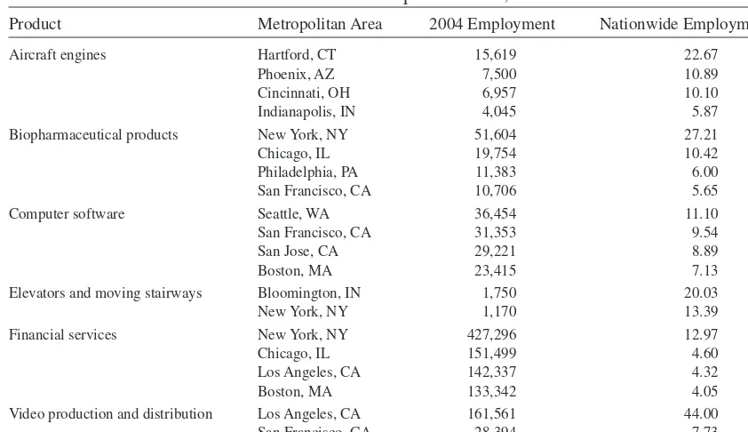
III. Why Do Firms Cluster?
This section analyzes the clustering of firms, highlighting the benefits of agglomeration such as sharing intermediate inputs and labor pooling. It discusses how self-reinforcing effects lead to industry clusters and the implications of these dynamics for urban economies. This knowledge equips students with a deeper understanding of economic geography and the strategic decisions of firms in urban settings.
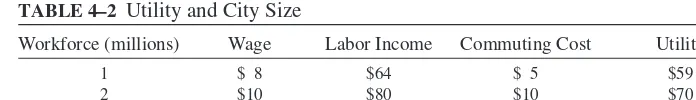
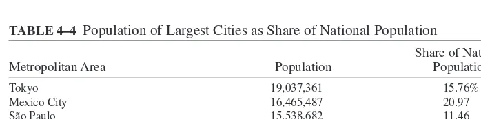
IV. City Size
This chapter explores the factors influencing city size, including utility, economic benefits, and costs associated with larger cities. It introduces models that explain the distribution of city sizes and discusses the implications of urban giants. Understanding city size is essential for students to analyze urban growth patterns and their economic consequences.
V. Urban Growth
Focusing on economic growth and its relationship to urban development, this chapter examines factors such as human capital, labor demand, and public policy. It discusses the impacts of urban growth on employment and income. This analysis provides students with the tools to evaluate urban economic policies and their effectiveness in fostering growth.
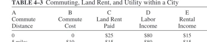
VI. Urban Land Rent
This section introduces the concept of land rent and its determinants, including bid-rent curves for different sectors. It explains how land use is shaped by economic forces and location decisions. By understanding land rent dynamics, students can better assess the implications for urban development and housing markets.
VII. Land-Use Patterns
This chapter investigates the spatial distribution of employment and population within urban areas. It explores the evolution from monocentric to decentralized cities and the implications for urban sprawl. This knowledge is critical for students to understand land-use planning and the socio-economic factors influencing urban form.
VIII. Neighborhood Choice
This section delves into the factors influencing neighborhood choice, including public goods, segregation, and externalities. It discusses the implications of these choices on urban dynamics and social equity. Understanding neighborhood dynamics is essential for students to address urban issues related to diversity and community development.
IX. Zoning and Growth Controls
This chapter examines the role of zoning laws and growth controls in shaping urban development. It discusses the history of zoning and its implications for land use and environmental policy. Students learn the importance of regulatory frameworks in urban planning and the trade-offs involved in growth management.
X. Autos and Highways
This section focuses on transportation's role in urban economies, particularly the effects of congestion and the costs associated with automobile use. It discusses potential solutions like congestion taxes and their implications for urban growth. This knowledge is vital for students to evaluate transportation policies and their impact on urban livability.
XI. Urban Transit
This chapter explores urban transit systems, analyzing ridership, costs, and the rationale for transit subsidies. It compares different transit modalities and their implications for urban land use. Understanding transit systems is crucial for students to develop effective urban mobility solutions and assess public transportation policies.
XII. Education
This section examines the economics of education in urban settings, focusing on the education production function and the impact of various inputs on educational outcomes. It discusses spending inequalities and policy implications. This knowledge is essential for students to understand the relationship between education and urban development.
XIII. Crime
This chapter discusses the economic aspects of urban crime, exploring its costs, causes, and prevention strategies. It analyzes the relationship between crime, poverty, and education. Understanding crime dynamics is vital for students to develop effective urban policies aimed at enhancing safety and community well-being.
XIV. Why Is Housing Different?
This section highlights the unique characteristics of the housing market, including heterogeneity and durability. It discusses the filtering model and the implications of housing policies. Students learn the nuances of the housing market, which is essential for effective urban policy and planning.
XV. Housing Policy
This chapter reviews various housing policies, including public housing, subsidies, and rent control. It evaluates their effectiveness and impact on the housing market. Understanding housing policy is crucial for students to formulate strategies that address urban housing challenges and promote equitable access.
XVI. The Role of Local Government
This section examines the functions of local government in urban economies, focusing on public goods and taxation. It discusses the Tiebout model and its implications for local governance. Understanding local government dynamics is essential for students to engage in effective urban policy-making.
XVII. Local Government Revenue
This chapter explores the revenue sources for local governments, including property taxes and intergovernmental grants. It discusses the implications for public service provision and fiscal policy. Students learn the importance of local government finance in shaping urban development and public policy.
XVIII.Appendix: Tools of Microeconomics
This appendix provides a review of key microeconomic concepts relevant to urban economics. It serves as a resource for students needing to refresh their understanding of economic principles. Mastery of these concepts is essential for students to effectively engage with the material presented throughout the book.
Referensi Dokumen
- Moral and Crime ( Moody, Carlisle E. )
- Economics of Mohring ( Mohring, Herbert )
- Moving to Opportunity (MTO) ( MTO )
- Education vouchers ( Murray, Sheila E. )
- Public Safety Programs ( Oates, Wallace E. )