All Your Biases Belong To Us:
Breaking RC4 in WPA-TKIP and TLS
Mathy Vanhoef
KU Leuven
[email protected]
Frank Piessens
KU Leuven
[email protected]
Abstract
We present new biases in RC4, break the Wi-Fi Protected Access Temporal Key Integrity Protocol (WPA-TKIP), and design a practical plaintext recovery attack against the Transport Layer Security (TLS) protocol. To empir-ically find new biases in the RC4 keystream we use sta-tistical hypothesis tests. This reveals many new biases in the initial keystream bytes, as well as several new long-term biases. Our fixed-plaintext recovery algorithms are capable of using multiple types of biases, and return a list of plaintext candidates in decreasing likelihood.
To break WPA-TKIP we introduce a method to gen-erate a large number of identical packets. This packet is decrypted by generating its plaintext candidate list, and using redundant packet structure to prune bad candidates. From the decrypted packet we derive the TKIP MIC key, which can be used to inject and decrypt packets. In prac-tice the attack can be executed within an hour. We also attack TLS as used by HTTPS, where we show how to decrypt a secure cookie with a success rate of 94% using 9·227ciphertexts. This is done by injecting known data around the cookie, abusing this using Mantin’sABSAB bias, and brute-forcing the cookie by traversing the plain-text candidates. Using our traffic generation technique, we are able to execute the attack in merely 75 hours.
1
Introduction
RC4 is (still) one of the most widely used stream ciphers. Arguably its most well known usage is in SSL and WEP, and in their successors TLS [8] and WPA-TKIP [19]. In particular it was heavily used after attacks against CBC-mode encryption schemes in TLS were published, such as BEAST [9], Lucky 13 [1], and the padding oracle at-tack [7]. As a mitigation RC4 was recommended. Hence, at one point around 50% of all TLS connections were us-ing RC4 [2], with the current estimate around 30% [18]. This motivated the search for new attacks, relevant ex-amples being [2, 20, 31, 15, 30]. Of special interest is
the attack proposed by AlFardan et al., where roughly 13·230ciphertexts are required to decrypt a cookie sent over HTTPS [2]. This corresponds to about 2000 hours of data in their setup, hence the attack is considered close to being practical. Our goal is to see how far these attacks can be pushed by exploring three areas. First, we search for new biases in the keystream. Second, we improve fixed-plaintext recovery algorithms. Third, we demon-strate techniques to perform our attacks in practice.
First we empirically search for biases in the keystream. This is done by generating a large amount of keystream, and storing statistics about them in several datasets. The resulting datasets are then analysed using statistical hy-pothesis tests. Our null hyhy-pothesis is that a keystream byte is uniformly distributed, or that two bytes are in-dependent. Rejecting the null hypothesis is equivalent to detecting a bias. Compared to manually inspecting graphs, this allows for a more large-scale analysis. With this approach we found many new biases in the initial keystream bytes, as well as several new long-term biases. We break WPA-TKIP by decrypting a complete packet using RC4 biases and deriving the TKIP MIC key. This key can be used to inject and decrypt packets [48]. In par-ticular we modify the plaintext recovery attack of Pater-son et al. [31, 30] to return a list of candidates in decreas-ing likelihood. Bad candidates are detected and pruned based on the (decrypted) CRC of the packet. This in-creases the success rate of simultaneously decrypting all unknown bytes. We achieve practicality using a novel method to rapidly inject identical packets into a network. In practice the attack can be executed within an hour.
the unknown cookie. We then generate a list of (cookie) candidates in decreasing likelihood, and use this to brute-force the cookie in negligible time. The algorithm to gen-erate candidates differs from the WPA-TKIP one due to the reliance on double-byte instead of single-byte likeli-hoods. All combined, we need 9·227 encryptions of a
cookie to decrypt it with a success rate of 94%. Finally we show how to make a victim generate this amount within only 75 hours, and execute the attack in practice.
To summarize, our main contributions are:
• We use statistical tests to empirically detect biases in the keystream, revealing large sets of new biases.
• We design plaintext recovery algorithms capable of using multiple types of biases, which return a list of plaintext candidates in decreasing likelihood.
• We demonstrate practical exploitation techniques to break RC4 in both WPA-TKIP and TLS.
The remainder of this paper is organized as follows. Section 2 gives a background on RC4, TKIP, and TLS. In Sect. 3 we introduce hypothesis tests and report new biases. Plaintext recovery techniques are given in Sect. 4. Practical attacks on TKIP and TLS are presented in Sect. 5 and Sect. 6, respectively. Finally, we summarize related work in Sect. 7 and conclude in Sect. 8.
2
Background
We introduce RC4 and its usage in TLS and WPA-TKIP.
2.1
The RC4 Algorithm
The RC4 algorithm is intriguingly short and known to be very fast in software. It consists of a Key Scheduling Algorithm (KSA) and a Pseudo Random Generation Al-gorithm (PRGA), which are both shown in Fig. 1. The state consists of a permutationSof the set{0, . . . ,255}, a public counteri, and a private index j. The KSA takes as input a variable-length key and initializesS. At each roundr=1,2, . . .of the PRGA, the yield statement out-puts a keystream byteZr. All additions are performed
modulo 256. A plaintext bytePr is encrypted to
cipher-text byteCrusingCr=Pr⊕Zr.
2.1.1 Short-Term Biases
Several biases have been found in the initial RC4 key-stream bytes. We call these short-term biases. The most significant one was found by Mantin and Shamir. They showed that the second keystream byte is twice as likely to be zero compared to uniform [25]. Or more formally that Pr[Z2=0]≈2·2−8, where the probability is over the
Listing (1) RC4 Key Scheduling (KSA).
1j, S = 0, range(256)
2for i in range(256):
3 j += S[i] + key[i % len(key)]
4 swap(S[i], S[j])
5return S
Listing (2) RC4 Keystream Generation (PRGA).
1S, i, j = KSA(key), 0, 0
2while True:
3 i += 1
4 j += S[i]
5 swap(S[i], S[j])
6 yield S[S[i] + S[j]]
Figure 1: Implementation of RC4 in Python-like pseudo-code. All additions are performed modulo 256.
random choice of the key. Because zero occurs more of-ten than expected, we call this a positive bias. Similarly, a value occurring less often than expected is called a neg-ative bias. This result was extended by Maitra et al. [23] and further refined by Sen Gupta et al. [38] to show that there is a bias towards zero for most initial keystream bytes. Sen Gupta et al. also found key-length dependent biases: ifℓis the key length, keystream byteZℓhas a pos-itive bias towards 256−ℓ[38]. AlFardan et al. showed that all initial 256 keystream bytes are biased by empiri-cally estimating their probabilities when 16-byte keys are used [2]. While doing this they found additional strong biases, an example being the bias towards valuerfor all positions 1≤r≤256. This bias was also independently discovered by Isobe et al. [20].
The bias Pr[Z1=Z2] =2−8(1−2−8)was found by
Paul and Preneel [33]. Isobe et al. refined this result for the value zero to Pr[Z1=Z2=0]≈3·2−16 [20].
In [20] the authors searched for biases of similar strength between initial bytes, but did not find additional ones. However, we did manage to find new ones (see Sect. 3.3).
2.1.2 Long-Term Biases
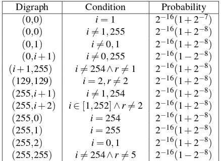
In contrast to short-term biases, which occur only in the initial keystream bytes, there are also biases that keep occurring throughout the whole keystream. We call these long-term biases. For example, Fluhrer and Mc-Grew (FM) found that the probability of certain digraphs, i.e., consecutive keystream bytes(Zr,Zr+1), deviate from
Digraph Condition Probability (0,0) i=1 2−16(1+2−7)
(0,0) i6=1,255 2−16(1+2−8)
(0,1) i6=0,1 2−16(1+2−8)
(0,i+1) i6=0,255 2−16(1−2−8) (i+1,255) i6=254∧r=6 1 2−16(1+2−8)
(129,129) i=2,r6=2 2−16(1+2−8)
(255,i+1) i6=1,254 2−16(1+2−8)
(255,i+2) i∈[1,252]∧r=6 2 2−16(1+2−8)
(255,0) i=254 2−16(1+2−8)
(255,1) i=255 2−16(1+2−8)
(255,2) i=0,1 2−16(1+2−8)
(255,255) i6=254∧r=6 5 2−16(1−2−8)
Table 1: Generalized Fluhrer-McGrew (FM) biases. Hereiis the public counter in the PRGA andrthe posi-tion of the first byte of the digraph. Probabilities for long-term biases are shown (for short-long-term biases see Fig. 4).
This assumption is only true after a few rounds of the PRGA [13, 26, 38]. Consequently these biases were gen-erally not expected to be present in the initial keystream bytes. However, in Sect. 3.3.1 we show that most of these biases do occur in the initial keystream bytes, albeit with different probabilities than their long-term variants.
Another long-term bias was found by Mantin [24]. He discovered a bias towards the patternABSAB, whereA andB represent byte values, andS a short sequence of bytes called the gap. With the length of the gapS de-noted byg, the bias can be written as:
Pr[(Zr,Zr+1) = (Zr+g+2,Zr+g+3)] =2−16(1+2−8e
−4−8g
256 )
(1) Hence the bigger the gap, the weaker the bias. Finally, Sen Gupta et al. found the long-term bias [38]
Pr[(Zw256,Zw256+2) = (0,0)] =2−16(1+2−8)
wherew≥1. We discovered that a bias towards(128,0) is also present at these positions (see Sect. 3.4).
2.2
TKIP Cryptographic Encapsulation
The design goal of WPA-TKIP was for it to be a tem-porary replacement of WEP [19, §11.4.2]. While it is being phased out by the WiFi Alliance, a recent study shows its usage is still widespread [48]. Out of 6803 net-works, they found that 71% of protected networks still allow TKIP, with 19% exclusively supporting TKIP.
Our attack on TKIP relies on two elements of the pro-tocol: its weak Message Integrity Check (MIC) [44, 48], and its faulty per-packet key construction [2, 15, 31, 30]. We briefly introduce both aspects, assuming a 512-bit
header TSC SNAP IP TCP MIC ICV
encrypted payload
Figure 2: Simplified TKIP frame with a TCP payload.
Pairwise Transient Key (PTK) has already been nego-tiated between the Access Point (AP) and client. From this PTK a 128-bit temporal encryption key (TK) and two 64-bit Message Integrity Check (MIC) keys are de-rived. The first MIC key is used for AP-to-client commu-nication, and the second for the reverse direction. Some works claim that the PTK, and its derived keys, are re-newed after a user-defined interval, commonly set to 1 hour [44, 48]. However, we found that generally only the Groupwise Transient Key (GTK) is periodically re-newed. Interestingly, our attack can be executed within an hour, so even networks which renew the PTK every hour can be attacked.
When the client wants to transmit a payload, it first calculates a MIC value using the appropriate MIC key and the Micheal algorithm (see Fig. Figure 2). Unfortu-nately Micheal is straightforward to invert: given plain-text data and its MIC value, we can efficiently derive the MIC key [44]. After appending the MIC value, a CRC checksum called the Integrity Check Value (ICV) is also appended. The resulting packet, including MAC header and example TCP payload, is shown in Figure 2. The payload, MIC, and ICV are encrypted using RC4 with a per-packet key. This key is calculated by a mixing function that takes as input the TK, the TKIP sequence counter (TSC), and the transmitter MAC address (TA). We write this as K=KM(TA,TK,TSC). The TSC is a 6-byte counter that is incremented after transmitting a packet, and is included unencrypted in the MAC header. In practice the output of KM can be modelled as uni-formly random [2, 31]. In an attempt to avoid weak-key attacks that broke WEP [12], the first three bytes of K are set to [19,§11.4.2.1.1]:
K0=TSC1 K1= (TSC1|0x20)& 0x7f K2=TSC0
Here, TSC0and TSC1are the two least significant bytes
of the TSC. Since the TSC is public, so are the first three bytes ofK. Both formally and using simulations, it has been shown this actually weakens security [2, 15, 31, 30].
2.3
The TLS Record Protocol
type version length payload HMAC
header RC4 encrypted
Figure 3: TLS Record structure when using RC4.
To send an encrypted payload, a TLS record of type application data is created. It contains the protocol ver-sion, length of the encrypted content, the payload itself, and finally an HMAC. The resulting layout is shown in Fig. 3. The HMAC is computed over the header, a se-quence number incremented for each transmitted record, and the plaintext payload. Both the payload and HMAC are encrypted. At the start of a connection, RC4 is ini-tialized with a key derived from the TLS master secret. This key can be modelled as being uniformly random [2]. None of the initial keystream bytes are discarded.
In the context of HTTPS, one TLS connection can be used to handle multiple HTTP requests. This is called a persistent connection. Slightly simplified, a server indi-cates support for this by setting the HTTPConnection header tokeep-alive. This implies RC4 is initialized only once to send all HTTP requests, allowing the usage of long-term biases in attacks. Finally, cookies can be marked as beingsecure, assuring they are transmitted only over a TLS connection.
3
Empirically Finding New Biases
In this section we explain how to empirically yet soundly detect biases. While we discovered many biases, we will not use them in our attacks. This simplifies the descrip-tion of the attacks. And, while using the new biases may improve our attacks, using existing ones already sufficed to significantly improve upon existing attacks. Hence our focus will mainly be on the most intriguing new biases.
3.1
Soundly Detecting Biases
In order to empirically detect new biases, we rely on hy-pothesis tests. That is, we generate keystream statistics over random RC4 keys, and use statistical tests to un-cover deviations from uniform. This allows for a large-scale and automated analysis. To detect single-byte bi-ases, our null hypothesis is that the keystream byte values are uniformly distributed. To detect biases between two bytes, one may be tempted to use as null hypothesis that the pair is uniformly distributed. However, this falls short if there are already single-byte biases present. In this case single-byte biases imply that the pair is also biased, while both bytes may in fact be independent. Hence, to detect double-byte biases, our null hypothesis is that they are independent. With this test, we even detected pairs
that are actually more uniform than expected. Rejecting the null hypothesis is now the same as detecting a bias.
To test whether values are uniformly distributed, we use a chi-squared goodness-of-fit test. A naive approach to test whether two bytes are independent, is using a chi-squared independence test. Although this would work, it is not ideal when only a few biases (outliers) are present. Moreover, based on previous work we expect that only a few values between keystream bytes show a clear de-pendency on each other [13, 24, 20, 38, 4]. Taking the Fluhrer-McGrew biases as an example, at any position at most 8 out of a total 65536 value pairs show a clear bias [13]. When expecting only a few outliers, the M-test of Fuchs and Kenett can be asymptotically more pow-erful than the chi-squared test [14]. Hence we use the M-test to detect dependencies between keystream bytes. To determine which values are biased between dependent bytes, we perform proportion tests over all value pairs.
We reject the null hypothesis only if the p-value is lower than 10−4. Holm’s method is used to control the family-wise error rate when performing multiple hypoth-esis tests. This controls the probability of even a single false positive over all hypothesis tests. We always use the two-sided variant of an hypothesis test, since a bias can be either positive or negative.
Simply giving or plotting the probability of two depen-dent bytes is not ideal. After all, this probability includes the single-byte biases, while we only want to report the strength of the dependency between both bytes. To solve this, we report the absolute relative bias compared to the expected single-byte based probability. More precisely, say that by multiplying the two single-byte probabilities of a pair, we would expect it to occur with probability p. Given that this pair actually occurs with probabilitys, we then plot the value|q|from the formulas=p·(1+q). In a sense the relative bias indicates how much information is gained by not just considering the single-byte biases, but using the real byte-pair probability.
3.2
Generating Datasets
In order to generate detailed statistics of keystream bytes, we created a distributed setup. We used roughly 80 stan-dard desktop computers and three powerful servers as workers. The generation of the statistics is done in C. Python was used to manage the generated datasets and control all workers. On start-up each worker generates a cryptographically random AES key. Random 128-bit RC4 keys are derived from this key using AES in counter mode. Finally, we used R for all statistical analysis [34]. Our main results are based on two datasets, called first16 and consec512. The first16 dataset esti-mates Pr[Za=x∧Zb=y]for 1≤a≤16, 1≤b≤256,
Digraph position
Absolute relativ
e bias
2−8.5 2−8 2−7.5 2−7 2−6.5
1 32 64 96 128 160 192 224 256 288
(0, 0) (0, 1) (0,i+1)
( i+1,255) (255, i+1) (255, i+2) (255,255)
Figure 4: Absolute relative bias of several Fluhrer-McGrew digraphs in the initial keystream bytes, com-pared to their expected single-byte based probability.
roughly 9 CPU years. This allows detecting biases be-tween the first 16 bytes and the other initial 256 bytes. Theconsec512dataset estimates Pr[Zr=x∧Zr+1=y]
for 1≤r≤512 and 0≤x,y<256 using 245keys, which took 16 CPU years to generate. It allows a detailed study of consecutive keystream bytes up to position 512.
We optimized the generation of both datasets. The first optimization is that one run of a worker generates at most 230keystreams. This allows usage of 16-bit
inte-gers for all counters collecting the statistics, even in the presence of significant biases. Only when combining the results of workers are larger integers required. This low-ers memory usage, reducing cache misses. To further re-duce cache misses we generate several keystreams before updating the counters. In independent work, Paterson et al. used similar optimizations [30]. For thefirst16 dataset we used an additional optimization. Here we first generate several keystreams, and then update the coun-ters in a sorted manner based on the value ofZa. This
optimization caused the most significant speed-up for the first16dataset.
3.3
New Short-Term Biases
By analysing the generated datasets we discovered many new short-term biases. We classify them into several sets.
3.3.1 Biases in (Non-)Consecutive Bytes
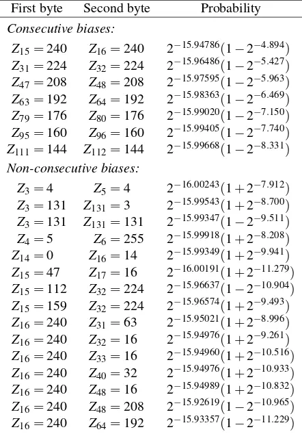
By analysing theconsec512dataset we discovered nu-merous biases between consecutive keystream bytes. Our first observation is that the Fluhrer-McGrew biases are also present in the initial keystream bytes. Excep-tions occur at posiExcep-tions 1, 2 and 5, and are listed in
Ta-First byte Second byte Probability Consecutive biases:
Z15=240 Z16=240 2−15.94786(1−2−4.894)
Z31=224 Z32=224 2−15.96486(1−2−5.427)
Z47=208 Z48=208 2−15.97595(1−2−5.963)
Z63=192 Z64=192 2−15.98363(1−2−6.469)
Z79=176 Z80=176 2−15.99020(1−2−7.150)
Z95=160 Z96=160 2−15.99405(1−2−7.740)
Z111=144 Z112=144 2−15.99668(1−2−8.331)
Non-consecutive biases:
Z3=4 Z5=4 2−16.00243(1+2−7.912)
Z3=131 Z131=3 2−15.99543(1+2−8.700)
Z3=131 Z131=131 2−15.99347(1−2−9.511)
Z4=5 Z6=255 2−15.99918(1+2−8.208)
Z14=0 Z16=14 2−15.99349(1+2−9.941)
Z15=47 Z17=16 2−16.00191(1+2−11.279)
Z15=112 Z32=224 2−15.96637(1−2−10.904)
Z15=159 Z32=224 2−15.96574(1+2−9.493)
Z16=240 Z31=63 2−15.95021(1+2−8.996)
Z16=240 Z32=16 2−15.94976(1+2−9.261)
Z16=240 Z33=16 2−15.94960(1+2−10.516)
Z16=240 Z40=32 2−15.94976(1+2−10.933)
Z16=240 Z48=16 2−15.94989(1+2−10.832)
Z16=240 Z48=208 2−15.92619(1−2−10.965)
Z16=240 Z64=192 2−15.93357(1−2−11.229)
Table 2: Biases between (non-consecutive) bytes.
ble 1 (note the extra conditions on the positionr). This is surprising, as the Fluhrer-McGrew biases were gener-ally not expected to be present in the initial keystream bytes [13]. However, these biases are present, albeit with different probabilities. Figure 4 shows the absolute rela-tive bias of most Fluhrer-McGrew digraphs, compared to their expected single-byte based probability (recall Sect. 3.1). For all digraphs, the sign of the relative biasq is the same as its long-term variant as listed in Table 1. We observe that the relative biases converge to their long-term values, especially after position 257. The vertical lines around position 1 and 256 are caused by digraphs which do not hold (or hold more strongly) around these positions.
A second set of strong biases have the form:
Pr[Zw16−1=Zw16=256−w16] (2)
with 1≤w≤7. In Table 2 we list their probabilities. Since 16 equals our key length, these are likely key-length dependent biases.
Another set of biases have the form Pr[Zr=Zr+1=x].
informa-Position other keystream byte (variable i)
Absolute relativ
e bias
2−11 2−10 2−9 2−8 2−7
1 32 64 96 128 160 192 224 256
Bias 1 Bias 3 Bias 5
Bias 2 Bias 4 Bias 6
Figure 5: Biases induced by the first two bytes. The num-ber of the biases correspond to those in Sect. 3.3.2.
tion. In principle, these biases also include the Fluhrer-McGrew pairs (0,0) and (255,255). However, as the bias for both these pairs is much higher than for other values, we don’t include them here. Our new bias, in the form of Pr[Zr=Zr+1], was detected up to position 512.
We also detected biases between non-consecutive bytes that do not fall in any obvious categories. An overview of these is given in Table 2. We remark that the biases induced byZ16=240 generally have a position,
or value, that is a multiple of 16. This is an indication that these are likely key-length dependent biases.
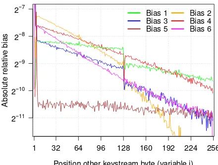
3.3.2 Influence ofZ1andZ2
Arguably our most intriguing finding is the amount of information the first two keystream bytes leak. In partic-ular,Z1andZ2influence all initial 256 keystream bytes.
We detected the following six sets of biases:
1) Z1=257−i∧Zi=0 4) Z1=i−1∧Zi=1
2) Z1=257−i∧Zi=i 5) Z2=0∧Zi=0
3) Z1=257−i∧Zi=257−i 6) Z2=0∧Zi=i
Their absolute relative bias, compared to the single-byte biases, is shown in Fig. 5. The relative bias of pairs 5 and 6, i.e., those involving Z2, are generally negative.
Pairs involvingZ1are generally positive, except pair 3,
which always has a negative relative bias. We also de-tected dependencies betweenZ1 andZ2 other than the
Pr[Z1=Z2] bias of Paul and Preneel [33]. That is, the
following pairs are strongly biased:
A)Z1=0∧Z2=x C)Z1=x∧Z2=0
B)Z1=x∧Z2=258−x D)Z1=x∧Z2=1
Bias A and C are negative for all x6=0, and both ap-pear to be mainly caused by the strong positive bias
Keystream byte value 0.00390577
0.00390589 0.00390601 0.00390613 0.00390625 0.00390637 0.00390649
0 32 64 96 128 160 192 224 256
Probability Position 272
Position 304 Position 336 Position 368
Figure 6: Single-byte biases beyond position 256.
Pr[Z1=Z2=0]found by Isobe et al. Bias B and D are
positive. We also discovered the following three biases:
Pr[Z1=Z3] =2−8(1−2−9.617) (3)
Pr[Z1=Z4] =2−8(1+2−8.590) (4)
Pr[Z2=Z4] =2−8(1−2−9.622) (5)
Note that all either involve an equality withZ1orZ2.
3.3.3 Single-Byte Biases
We analysed single-byte biases by aggregating the consec512dataset, and by generating additional statis-tics specifically for single-byte probabilities. The aggre-gation corresponds to calculating
Pr[Zr=k] = 255
∑
y=0
Pr[Zr=k∧Zr+1=y] (6)
We ended up with 247keys used to estimate single-byte probabilities. For all initial 513 bytes we could reject the hypothesis that they are uniformly distributed. In other words, all initial 513 bytes are biased. Figure 6 shows the probability distribution for some positions. Manual inspection of the distributions revealed a significant bias towardsZ256+k·16=k·32 for 1≤k≤7. These are likely
key-length dependent biases. Following [26] we conjec-ture there are single-byte biases even beyond these posi-tions, albeit less strong.
3.4
New Long-Term Biases
To search for new long-term biases we created a variant of thefirst16dataset. It estimates
Pr[Z256w+a=x∧Z256w+b=y] (7)
dropped the initial 1023 keystream bytes. Using this dataset we can detect biases whose periodicity is a proper divisor of 256 (e.g., it detected all Fluhrer-McGrew bi-ases). Our new short-term biases were not present in this dataset, indicating they indeed only occur in the initial keystream bytes, at least with the probabilities we listed. We did find the new long-term bias
Pr[(Zw256,Zw256+2) = (128,0)] =2−16(1+2−8) (8)
forw≥1. Surprisingly this was not discovered earlier, since a bias towards(0,0)at these positions was already known [38]. We also specifically searched for biases of the form Pr[Zr=Zr′]by aggregating our dataset. This
revealed that many bytes are dependent on each other. That is, we detected several long-term biases of the form
Pr[Z256w+a=Z256w+b]≈2−8(2±2−16) (9)
Due to the small relative bias of 2−16, these are difficult
to reliably detect. That is, the pattern where these biases occur, and when their relative bias is positive or nega-tive, is not yet clear. We consider it an interesting future research direction to (precisely and reliably) detect all keystream bytes which are dependent in this manner.
4
Plaintext Recovery
We will design plaintext recovery techniques for usage in two areas: decrypting TKIP packets and HTTPS cookies. In other scenarios, variants of our methods can be used.
4.1
Calculating Likelihood Estimates
Our goal is to convert a sequence of ciphertextsC into predictions about the plaintext. This is done by exploit-ing biases in the keystream distributionspk=Pr[Zr=k].
These can be obtained by following the steps in Sect. 3.2. All biases in pkare used to calculate the likelihood that
a plaintext byte equals a certain value µ. To accom-plish this, we rely on the likelihood calculations of Al-Fardan et al. [2]. Their idea is to calculate, for each plaintext valueµ, the (induced) keystream distributions required to witness the captured ciphertexts. The closer this matches the real keystream distributionspk, the more
likely we have the correct plaintext byte. Assuming a fixed positionrfor simplicity, the induced keystream dis-tributions are defined by the vectorNµ= (N0µ, . . . ,N255µ ). EachNkµ represents the number of times the keystream byte was equal tok, assuming the plaintext byte wasµ:
Nkµ =|{C∈ C |C=k⊕µ}| (10)
Note that the vectors Nµ and Nµ′ are permutations of each other. Based on the real keystream probabilitiespk
we calculate the likelihood that this induced distribution would occur in practice. This is modelled using a multi-nomial distribution with the number of trails equal to|C|, and the categories being the 256 possible keystream byte values. Since we want the probability of thissequenceof keystream bytes we get [30]:
Pr[C |P=µ] =
∏
k∈{0,...,255} (pk)N
µ
k (11)
Using Bayes’ theorem we can convert this into the like-lihoodλµ that the plaintext byte isµ:
λµ=Pr[P=µ| C]∼Pr[C |P=µ] (12)
For our purposes we can treat this as an equality [2]. The most likely plaintext byteµis the one that maximisesλµ.
This was extended to a pair of dependent keystream bytes in the obvious way:
λµ1,µ2=
∏
k1,k2∈{0,...,255}
(pk1,k2)
Nµ1,µ2
k1,k2 (13)
We found this formula can be optimized if most key-stream byte values k1 andk2are independent and
uni-form. More precisely, let us assume that all keystream value pairs in the setIare independent and uniform:
∀(k1,k2)∈ I: pk1,k2=pk1·pk2=u (14)
whereurepresents the probability of an unbiased double-byte keystream value. Then we rewrite formula 13 to:
λµ1,µ2= (u)
Mµ1,µ2
·
∏
k1,k2∈Ic
(pk1,k2)
Nkµ1,µ2
1,k2 (15)
where
Mµ1,µ2=
∑
k1,k2∈I
Nµ1,µ2
k1,k2 =|C| −
∑
k1,k2∈Ic
Nµ1,µ2
k1,k2 (16)
and withIcthe set of dependent keystream values. If the
setIc is small, this results in a lower time-complexity.
For example, when applied to the long-term keystream setting over Fluhrer-McGrew biases, roughly 219 opera-tions are required to calculate all likelihood estimates, in-stead of 232. A similar (though less drastic) optimization
can also be made when single-byte biases are present.
4.2
Likelihoods From Mantin’s Bias
We now show how to compute a double-byte plaintext likelihood using Mantin’sABSABbias. More formally, we want to compute the likelihoodλµ1,µ2 that the
plain-text bytes at fixed positions randr+1 areµ1andµ2,
likelihood of thedifferentialbetween the known and un-known plaintext. We define the differentialZbrgas:
b
Zrg= (Zr⊕Zr+2+g,Zr+1⊕Zr+3+g) (17)
Similarly we useCbgr andPbrgto denote the differential over
ciphertext and plaintext bytes, respectively. TheABSAB bias can then be written as:
Pr[Zbrg= (0,0)] =2−16(1+2−8e−4256−8g) =α(g) (18)
When XORing both sides ofZbrg= (0,0)withPbrgwe get
Pr[Cbgr =Pbrg] =α(g) (19)
Hence Mantin’s bias implies that the ciphertext differen-tial is biased towards the plaintext differendifferen-tial. We use this to calculate the likelihoodλµbof a differentialbµ. For ease of notation we assume a fixed positionrand a fixed ABSABgap ofg. LetCbbe the sequence of captured ci-phertext differentials, andµ1′ andµ2′ the known plaintext bytes at positionsr+2+g andr+3+g, respectively. Similar to our previous likelihood estimates, we calcu-late the probability of witnessing the ciphertext differen-tialsCbassuming the plaintext differential isµb:
Pr[C |b Pb=µb] =
∏
bk∈{0,...,255}2
Pr[Zb=bk]Nbkµb (20)
where
Nbµb
k =
nCb∈C |b Cb=bk⊕bµo (21)
Using this notation we see that this is indeed identical to an ordinary likelihood estimation. Using Bayes’ theorem we getλµb=Pr[C |b Pb=µb]. Since only one differential pair is biased, we can apply and simplify formula 15:
λµb= (1−α(g))|C|−|bu|·α(g)|bµ| (22)
where we slightly abuse notation by defining|µb|as
|µb|=nCb∈C |b Cb=µbo (23)
Finally we apply our knowledge of the known plaintext bytes to get our desired likelihood estimate:
λµ1,µ2 =λbµ⊕(µ1′,µ2′) (24)
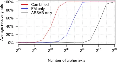
To estimate at which gap size theABSABbias is still detectable, we generated 248 blocks of 512 keystream bytes. Based on this we empirically confirmed Mantin’s ABSAB bias up to gap sizes of at least 135 bytes. The theoretical estimate in formula 1 slightly underestimates the true empirical bias. In our attacks we use a maximum gap size of 128.
Number of ciphertexts
A
ver
age reco
ver
y r
ate
0% 20% 40% 60% 80% 100%
227 229 231 233 235 237 239
Combined FM only ABSAB only
Figure 7: Average success rate of decrypting two bytes using: (1) oneABSABbias; (2) Fluhrer-McGrew (FM) biases; and (3) combination of FM biases with 258 ABSABbiases. Results based on 2048 simulations each.
4.3
Combining Likelihood Estimates
Our goal is to combine multiple types of biases in a likeli-hood calculation. Unfortunately, if the biases cover over-lapping positions, it quickly becomes infeasible to per-form a single likelihood estimation over all bytes. In the worst case, the calculation cannot be optimized by rely-ing on independent biases. Hence, a likelihood estimate overnkeystream positions would have a time complex-ity ofO(22·8·n). To overcome this problem, we perform
and combine multiple separate likelihood estimates. We will combine multiple types of biases by multi-plying their individual likelihood estimates. For exam-ple, let λµ′
1,µ2 be the likelihood of plaintext bytes µ1
andµ2based on the Fluhrer-McGrew biases. Similarly,
letλg′,µ1,µ2 be likelihoods derived fromABSABbiases of gapg. Then their combination is straightforward:
λµ1,µ2=λ
′
µ1,µ2·
∏
g
λg′,µ
1,µ2 (25)
While this method may not be optimal when combining likelihoods of dependent bytes, it does appear to be a general and powerful method. An open problem is de-termining which biases can be combined under a single likelihood calculation, while keeping computational re-quirements acceptable. Likelihoods based on other bi-ases, e.g., Sen Gupta’s and our new long-term bibi-ases, can be added as another factor (though some care is needed so positions properly overlap).
maximumABSABgap of 128 bytes. Figure 7 shows the results of this experiment. Notice that a singleABSAB bias is weaker than using all Fluhrer-McGrew biases at a specific position. However, combining severalABSAB biases clearly results in a major improvement. We con-clude that our approach to combine biases significantly reduces the required number of ciphertexts.
4.4
List of Plaintext Candidates
In practice it is useful to have a list of plaintext candi-dates in decreasing likelihood. For example, by travers-ing this list we could attempt to brute-force keys, pass-words, cookies, etc. (see Sect. 6). In other situations the plaintext may have a rigid structure allowing the removal of candidates (see Sect. 5). We will generate a list of plaintext candidates in decreasing likelihood, when given either single-byte or double-byte likelihood estimates.
First we show how to construct a candidate list when given single-byte plaintext likelihoods. While it is trivial to generate the two most likely candidates, beyond this point the computation becomes more tedious. Our solu-tion is to incrementally compute theN most likely can-didates based on their length. That is, we first compute theNmost likely candidates of length 1, then of length 2, and so on. Algorithm 1 gives a high-level implemen-tation of this idea. VariablePr[i] denotes thei-th most
likely plaintext of lengthr, having a likelihood ofEr[i].
The twominoperations are needed because in the initial loops we are not yet be able to generate N candidates, i.e., there only exist 256rplaintexts of lengthr. Picking the µ′ which maximizes pr(µ′)can be done efficiently using a priority queue. In practice, only the latest two versions of lists E andP need to be stored. To better maintain numeric stability, and to make the computation more efficient, we perform calculations using the loga-rithm of the likelihoods. We implemented Algologa-rithm 1 and report on its performance in Sect. 5, where we use it to attack a wireless network protected by WPA-TKIP.
To generate a list of candidates from double-byte like-lihoods, we first show how to model the likelihoods as a hidden Markov model (HMM). This allows us to present a more intuitive version of our algorithm, and refer to the extensive research in this area if more efficient im-plementations are needed. The algorithm we present can be seen as a combination of the classical Viterbi algo-rithm, and Algorithm 1. Even though it is not the most optimal one, it still proved sufficient to significantly im-prove plaintext recovery (see Sect. 6). For an introduc-tion to HMMs we refer the reader to [35]. Essentially an HMM models a system where the internal states are not observable, and after each state transition, output is (probabilistically) produced dependent on its new state.
We model the plaintext likelihood estimates as a
first-Algorithm 1: Generate plaintext candidates in de-creasing likelihood using single-byte estimates.
Input:L: Length of the unknown plaintext
λ1≤r≤L,0≤µ≤255: single-byte likelihoods
N: Number of candidates to generate
Returns: List of candidates in decreasing likelihood
P0[1]←ε
E0[1]←0
forr=1toLdo forµ=0to255do
pos(µ)←1
pr(µ)←Er−1[1] +log(λr,µ) fori=1tomin(N,256r)do
µ←µ′which maximizespr(µ′) Pr[i]←Pr−1[pos(µ)]kµ
Er[i]←Er−1[pos(µ)] +log(λr,µ)
pos(µ)←pos(µ) +1
pr(µ)←Er−1[pos(µ)] +log(λr,µ) ifpos(µ)>min(N,256r−1)then
pr(µ)← −∞
returnPN
order time-inhomogeneous HMM. The state spaceS of the HMM is defined by the set of possible plaintext val-ues{0, . . . ,255}. The byte positions are modelled using the time-dependent (i.e., inhomogeneous) state transition probabilities. Intuitively, the “current time” in the HMM corresponds to the current plaintext position. This means the transition probabilities for moving from one state to another, which normally depend on the current time, will now depend on the position of the byte. More formally:
Pr[St+1=µ2|St=µ1]∼λt,µ1,µ2 (26)
wheret represents the time. For our purposes we can treat this as an equality. In an HMM it is assumed that its current state is not observable. This corresponds to the fact that we do not know the value of any plaintext bytes. In an HMM there is also some form of output which depends on the current state. In our setting a par-ticular plaintext value leaks no observable (side-channel) information. This is modelled by always letting every state produce the same null output with probability one.
Algorithm 2: Generate plaintext candidates in de-creasing likelihood using double-byte estimates.
Input:L: Length of the unknown plaintext plus two m1andmL: known first and last byte
λ1≤r<L,0≤µ1,µ2≤255: double-byte likelihoods
N: Number of candidates to generate
Returns: List of candidates in decreasing likelihood
forµ2=0to255do
E2[µ2,1]←log(λ1,m1,µ2)
P2[µ2,1]←m1kµ2
forr=3toLdo forµ2=0to255do
forµ1=0to255do
pos(µ1)←1
pr(µ1)←Er−1[µ1,1] +log(λr,µ1,µ2)
fori=1tomin(N,256r−1)do
µ1←µwhich maximizespr(µ)
Pr[µ2,i]←Pr−1[µ1,pos(µ1)]kµ2
Er[µ2,i]←Er−1[µ1,pos(µ1)] +log(λr,µ1,µ2)
pos(µ1)←pos(µ1) +1
pr(µ1)←Er−1[µ1,pos(µ1)] +log(λr,µ1,µ2)
ifpos(µ1)>min(N,256r−2)then
pr(µ1)← −∞
returnPN[mL,:]
algorithm) can be used, examples being [42, 36, 40, 28]. The simplest form of such an algorithm keeps track of theNbest candidates ending in a particular valueµ, and is shown in Algorithm 2. Similar to [2, 30] we assume the first byte m1 and last byte mL of the plaintext are
known. During the last round of the outer for-loop, the loop overµ2has to be executed only for the valuemL. In
Sect. 6 we use this algorithm to generate a list of cookies. Algorithm 2 uses considerably more memory than Al-gorithm 1. This is because it has to store the N most likely candidates for each possible ending valueµ. We remind the reader that our goal is not to present the most optimal algorithm. Instead, by showing how to model the problem as an HMM, we can rely on related work in this area for more efficient algorithms [42, 36, 40, 28]. Since an HMM can be modelled as a graph, allk-shortest path algorithms are also applicable [10]. Finally, we remark that even our simple variant sufficed to significantly im-prove plaintext recovery rates (see Sect. 6).
5
Attacking WPA-TKIP
We use our plaintext recovery techniques to decrypt a full packet. From this decrypted packet the MIC key can be
derived, allowing an attacker to inject and decrypt pack-ets. The attack takes only an hour to execute in practice.
5.1
Calculating Plaintext Likelihoods
We rely on the attack of Paterson et al. to compute plain-text likelihood estimates [31, 30]. They noticed that the first three bytes of the per-packet RC4 key are public. As explained in Sect. 2.2, the first three bytes are fully determined by the TKIP Sequence Counter (TSC). It was observed that this dependency causes strong TSC-dependent biases in the keystream [31, 15, 30], which can be used to improve the plaintext likelihood estimates. For each TSC value they calculated plaintext likelihoods based on empirical, per-TSC, keystream distributions. The resulting 2562likelihoods, for one plaintext byte, are
combined by multiplying them over all TSC pairs. In a sense this is similar to combining multiple types of biases as done in Sect. 4.3, though here the different types of bi-ases are known to be independent. We use the single-byte variant of the attack [30,§4.1] to obtain likelihoodsλr,µ
for every unknown byte at a given positionr.
The downside of this attack is that it requires detailed per-TSC keystream statistics. Paterson at al. generated statistics for the first 512 bytes, which took 30 CPU years [30]. However, in our attack we only need these statistics for the first few keystream bytes. We used 232 keys per TSC value to estimate the keystream distribu-tion for the first 128 bytes. Using our distributed setup the generation of these statistics took 10 CPU years.
With our per-TSC keystream distributions we obtained similar results to that of Paterson et al. [31, 30]. By run-ning simulations we confirmed that the odd byte posi-tions [30], instead of the even ones [31], can be recov-ered with a higher probability than others. Similarly, the bytes at positions 49-51 and 63-67 are generally recov-ered with higher probability as well. Both observations will be used to optimize the attack in practice.
5.2
Injecting Identical Packets
such method is abusing the inclusion of (insecure) third-party resources on popular websites [27]. For example, an attacker can register a mistyped domain, accidentally used in a resource address (e.g., an image URL) on a popular website. Whenever the victim visits this website and loads the resource, a TCP connection is made to the server of the attacker. In [27] these types of vulnerabil-ities were found to be present on several popular web-sites. Additionally, any type of web vulnerability that can be abused to make a victim execute JavaScript can be utilised. In this sense, our requirements are more relaxed than those of the recent attacks on SSL and TLS, which requirethe ability to run JavaScript code in the victim’s browser [9, 1, 2]. Another method is to hijack an exist-ing TCP connection of the victim, which under certain conditions is possible without a man-in-the-middle posi-tion [17]. We conclude that, while there is no universal method to accomplish this, we can assume control over a TCP connection with the victim. Using this connection we inject identical packets by repeatedly retransmitting identical TCP packets. Since retransmissions are valid TCP behaviour, this will work even if the victim is be-hind a firewall.
We now determine the optimal structure of the injected packet. A naive approach would be to use the shortest possible packet, meaning no TCP payload is included. Since the total size of the LLC/SNAP, IP, and TCP header is 48 bytes, the MIC and ICV would be located at posi-tion 49 up to and including 60 (see Fig. 2). At these locations 7 bytes are strongly biased. In contrast, if we use a TCP payload of 7 bytes, the MIC and ICV are lo-cated at position 56 up to and including 60. In this range 8 bytes are strongly biased, resulting in better plaintext likelihood estimates. Through simulations we confirmed that using a 7 byte payload increases the probability of successfully decrypting the MIC and ICV. In practice, adding 7 bytes of payload also makes the length of our injected packet unique. As a result we can easily identify and capture such packets. Given both these advantages, we use a TCP data packet containing 7 bytes of payload.
5.3
Decrypting a Complete Packet
Our goal is to decrypt the injected TCP packet, including its MIC and ICV fields. Note that all these TCP packets will be encrypted with a different RC4 key. For now we assume all fields in the IP and TCP packet are known, and we will later show why we can safely make this as-sumption. Hence, only the 8-byte MIC and 4-byte ICV of the packet remain unknown. We use the per-TSC key-stream statistics to compute single-byte plaintext likeli-hoods for all 12 bytes. However, this alone would give a very low success probability of simultaneously (cor-rectly) decrypting all bytes. We solve this by realising
Ciphertext copies times 220
Probability MIC k
e
y reco
ver
y
0% 20% 40% 60% 80% 100%
1 3 5 7 9 11 13 15
230 candidates 2 candidates
Figure 8: Success rate of obtaining the TKIP MIC key using nearly 230candidates, and using only the two best candidates. Results are based on 256 simulations each.
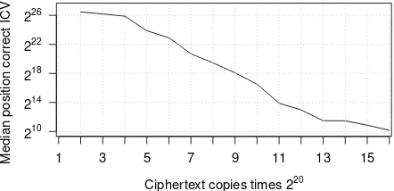
Ciphertext copies times 220
Median position correct ICV
210 214 218 222 226
1 3 5 7 9 11 13 15
Figure 9: Median position of a candidate with a correct ICV with nearly 230candidates. Results are based on 256 simulations each.
that the TKIP ICV is a simple CRC checksum which we can easily verify ourselves. Hence we can detect bad candidates by inspecting their CRC checksum. We now generate a plaintext candidate list, and traverse it until we find a packet having a correct CRC. This drastically im-proves the probability of simultaneously decrypting all bytes. From the decrypted packet we can derive the TKIP MIC key [44], which can then be used to inject and de-crypt arbitrary packets [48].
Figure 8 shows the success rate of finding a packet with a good ICV and deriving the correct MIC key. For comparison, it also includes the success rates had we only used the two most likely candidates. Figure 9 shows the median position of the first candidate with a correct ICV. We plot the median instead of average to lower in-fluence of outliers, i.e., at times the correct candidate was unexpectedly far (or early) in the candidate list.
success rates. This can be done independently of each other, and independently of decrypting the MIC and ICV. Another method to obtain the internal IP is to rely on HTML5 features. If the initial TCP connection is created by a browser, we can first send JavaScript code to obtain the internal IP of the victim using WebRTC [37]. We also noticed that our NAT gateway generally did not modify the source port used by the victim. Consequently we can simply read this value at the server. The TTL field can also be determined without relying on the IP checksum. Using atraceroutecommand we count the number of hops between the server and the client, allowing us to derive the TTL value at the victim.
5.4
Empirical Evaluation
To test the plaintext recovery phase of our attack we cre-ated a tool that parses a rawpcapfile containing the cap-tured Wi-Fi packets. It searches for the injected packets, extracts the ciphertext statistics, calculates plaintext like-lihoods, and searches for a candidate with a correct ICV. From this candidate, i.e., decrypted injected packet, we derive the MIC key.
For the ciphertext generation phase we used an OpenVZ VPS as malicious server. The incoming TCP connection from the victim is handled using a custom tool written in Scapy. It relies on a patched version of Tcpreplay to rapidly inject the identical TCP packets. The victim machine is a Latitude E6500 and is connected to an Asus RT-N10 router running Tomato 1.28. The victim opens a TCP connection to the malicious server by visiting a website hosted on it. For the attacker we used a Compaq 8510p with an AWUS036nha to capture the wireless traffic. Under this setup we were able to generate roughly 2500 packets per second. This number was reached even when the victim was actively brows-ing YouTube videos. Thanks to the 7-byte payload, we uniquely detected the injected packet in all experiments without any false positives.
We ran several test where we generated and captured traffic for (slightly more) than one hour. This amounted to, on average, capturing 9.5·220different encryptions of the packet being injected. Retransmissions were filtered based on the TSC of the packet. In nearly all cases we successfully decrypted the packet and derived the MIC key. Recall from Sect. 2.2 that this MIC key is valid as long as the victim does not renew its PTK, and that it can be used to inject and decrypt packets from the AP to the victim. For one capture our tool found a packet with a correct ICV, but this candidate did not correspond to the actual plaintext. While our current evaluation is limited in the number of captures performed, it shows the attack is practically feasible, with overall success probabilities appearing to agree with the simulated results of Fig. 8.
Listing 3: Manipulated HTTP request, with known plain-text surrounding the cookie at both sides.
1GET / HTTP/1.1
2Host: site.com
3User-Agent: Mozilla/5.0 (X11; Linux i686; rv:32.0)
Gecko/20100101 Firefox/32.0
4Accept: text/html,application/xhtml+xml,application/
xml;q=0.9,*/*;q=0.8
5Accept-Language: en-US,en;q=0.5
6Accept-Encoding: gzip, deflate
7Cookie: auth=XXXXXXXXXXXXXXXX; injected1=known1;
injected2=knownplaintext2; ...
6
Decrypting HTTPS Cookies
We inject known data around a cookie, enabling use of theABSABbiases. We then show that a HTTPS cookie can be brute-forced using only 75 hours of ciphertext.
6.1
Injecting Known Plaintext
We want to be able to predict the position of the targeted cookie in the encrypted HTTP requests, and surround it with known plaintext. To fix ideas, we do this for the se-cureauthcookie sent tohttps://site.com. Similar to previous attacks on SSL and TLS, we assume the at-tacker is able to execute JavaScript code in the victim’s browser [9, 1, 2]. In our case, this means an active man-in-the-middle (MiTM) position is used, where plaintext HTTP channels can be manipulated. Our first realisa-tion is that an attacker can predict the length and con-tent of HTTP headers preceding the Cookie field. By monitoring plaintext HTTP requests, these headers can be sniffed. If the targetedauthcookie is the first value in theCookieheader, this implies we know its position in the HTTP request. Hence, our goal is to have a layout as shown in Listing 3. Here the targeted cookie is the first value in theCookieheader, preceded by known headers, and followed by attacker injected cookies.
will be included after theauthcookie. An example of a HTTP(S) request manipulated in this manner is shown in Listing 3. Here the secureauthcookie is surrounded by known plaintext at both sides. This allows us to use Mantin’sABSABbias when calculating plaintext likeli-hoods.
6.2
Brute-Forcing The Cookie
In contrast to passwords, many websites do not protect against brute-forcing cookies. One reason for this is that the password of an average user has a much lower en-tropy than a random cookie. Hence it makes sense to brute-force a password, but not a cookie: the chance of successfully brute-forcing a (properly generated) cookie is close to zero. However, if RC4 can be used to con-nect to the web server, our candidate generation algo-rithm voids this assumption. We can traverse the plain-text candidate list in an attempt to brute-force the cookie. Since we are targeting a cookie, we can exclude cer-tain plaintext values. As RFC 6265 states, a cookie value can consists of at most 90 unique characters [3,§4.1.1]. A similar though less general observation was already made by AlFardan et al. [2]. Our observation allows us to give a tighter bound on the required number of cipher-texts to decrypt a cookie, even in the general case. In practice, executing the attack with a reduced character set is done by modifying Algorithm 2 so the for-loops overµ1andµ2only loop over allowed characters.
Figure 10 shows the success rate of brute-forcing a 16-character cookie using at most 223attempts. For
compar-ison, we also include the probability of decrypting the cookie if only the most likely plaintext was used. This also allows for an easier comparison with the work of AlFardan et al. [2]. Note that they only use the Fluhrer-McGrew biases, whereas we combine serveral ABSAB biases together with the Fluhrer-McGrew biases. We conclude that our brute-force approach, as well as the inclusion of the ABSAB biases, significantly improves success rates. Even when using only 223brute-force at-tempts, success rates of more than 94% are obtained once 9·227encryptions of the cookie have been captured. We conjecture that generating more candidates will further increase success rates.
6.3
Empirical Evaluation
The main requirement of our attack is being able to col-lect sufficiently many encryptions of the cookie, i.e., hav-ing many ciphertexts. We fulfil this requirement by forc-ing the victim to generate a large number of HTTPS re-quests. As in previous attacks on TLS [9, 1, 2], we ac-complish this by assuming the attacker is able to execute JavaScript in the browser of the victim. For example,
Ciphertext copies times 227
Probability successful br
ute−f
orce
0% 20% 40% 60% 80% 100%
1 3 5 7 9 11 13 15
223 candidates 1 candidate
Figure 10: Success rate of brute-forcing a 16-character cookie using roughly 223candidates, and only the most likely candidate, dependent on the number of collected ciphertexts. Results based on 256 simulations each.
when performing a man-the-middle attack, we can in-ject JavaScript into any plaintext HTTP connection. We then useXMLHttpRequestobjects to issue Cross-Origin Requests to the targeted website. The browser will auto-matically add the secure cookie to these (encrypted) re-quests. Due to the same-origin policy we cannot read the replies, but this poses no problem, we only require that the cookie is included in the request. The requests are sent inside HTML5 WebWorkers. Essentially this means our JavaScript code will run in the background of the browser, and any open page(s) stay responsive. We use GET requests, and carefully craft the values of our in-jected cookies so the targetedauth cookie is always at a fixed position in the keystream (modulo 256). Recall that this alignment is required to make optimal use of the Fluhrer-McGrew biases. An attacker can learn the re-quired amount of padding by first letting the client make a request without padding. Since RC4 is a stream cipher, and no padding is added by the TLS protocol, an attacker can easily observe the length of this request. Based on this information it is trivial to derive the required amount of padding.
To test our attack in practice we implemented a tool in C which monitors network traffic and collects the nec-essary ciphertext statistics. This requires reassembling the TCP and TLS streams, and then detecting the 512-byte (encrypted) HTTP requests. Similar to optimizing the generation of datasets as in Sect. 3.2, we cache sev-eral requests before updating the counters. We also cre-ated a tool to brute-force the cookie based on the gen-erated candidate list. It uses persistent connections and HTTP pipelining [11,§6.3.2]. That is, it uses one con-nection to send multiple requests without waiting for each response.
used. We use nginx as the web server, and configured RC4-SHA1 with RSA as the only allowable cipher suite. This assures that RC4 is used in all tests. Both the server and client use an Intel 82579LM network card, with the link speed set to 100 Mbps. With an idle browser this setup resulted in an average of 4450 requests per second. When the victim was actively browsing YouTube videos this decreased to roughly 4100. To achieve such num-bers, we found it’s essential that the browser uses persis-tent connections to transmit the HTTP requests. Other-wise a new TCP and TLS handshake must be performed for every request, whose round-trip times would signif-icantly slow down traffic generation. In practice this means the website must allow a keep-alive connec-tion. While generating requests the browser remained re-sponsive at all times. Finally, our custom tool was able to test more than 20000 cookies per second. To execute the attack with a success rate of 94% we need roughly 9·227 ciphertexts. With 4450 requests per seconds, this means we require 75 hours of data. Compared to the (more than) 2000 hours required by AlFardan et al. [2,§5.3.3] this is a significant improvement. We remark that, similar to the attack of AlFardan et al. [2], our attack also tolerates changes of the encryption keys. Hence, since cookies can have a long lifetime, the generation of this traffic can even be spread out over time. With 20000 brute-force at-tempts per second, all 223 candidates for the cookie can be tested in less than 7 minutes.
We have executed the attack in practice, and success-fully decrypted a 16-character cookie. In our instance, capturing traffic for 52 hours already proved to be suf-ficient. At this point we collected 6.2·227 ciphertexts. After processing the ciphertexts, the cookie was found at position 46229 in the candidate list. This serves as a good example that, if the attacker has some luck, less cipher-texts are needed than our 9·227estimate. These results
push the attack from being on the verge of practicality, to feasible, though admittedly somewhat time-consuming.
7
Related Work
Due to its popularity, RC4 has undergone wide crypt-analysis. Particularly well known are the key recovery attacks that broke WEP [12, 50, 45, 44, 43]. Several other key-related biases and improvements of the orig-inal WEP attack have also been studied [21, 39, 32, 22]. We refer to Sect. 2.1 for an overview of various biases discovered in the keystream [25, 23, 38, 2, 20, 33, 13, 24, 38, 15, 31, 30]. In addition to these, the long-term bias Pr[Zr=Zr+1|2·Zr=ir] =2−8(1+2−15)was
dis-covered by Basu et al. [4]. While this resembles our new short-term bias Pr[Zr=Zr+1], in their analysis they
as-sume the internal stateSis a random permutation, which is true only after a few rounds of the PRGA. Isobe et
al. searched for dependencies between initial keystream bytes by empirically estimating Pr[Zr=y∧Zr−a=x]for
0≤x,y≤255, 2≤r≤256, and 1≤a≤8 [20]. They did not discover any new biases using their approach. Mironov modelled RC4 as a Markov chain and recom-mended to skip the initial 12·256 keystream bytes [26]. Paterson et al. generated keystream statistics over con-secutive keystream bytes when using the TKIP key struc-ture [30]. However, they did not report which (new) bi-ases were present. Through empirical analysis, we show that biases between consecutive bytes are present even when using RC4 with random 128 bit keys.
The first practical attack on WPA-TKIP was found by Beck and Tews [44] and was later improved by other re-searchers [46, 16, 48, 49]. Recently several works stud-ied the per-packet key construction both analytically [15] and through simulations [2, 31, 30]. For our attack we replicated part of the results of Paterson et al. [31, 30], and are the first to demonstrate this type of attack in prac-tice. In [2] AlFardan et al. ran experiments where the two most likely plaintext candidates were generated us-ing sus-ingle-byte likelihoods [2]. However, they did not present an algorithm to return arbitrarily many candi-dates, nor extended this to double-byte likelihoods.
The SSL and TLS protocols have undergone wide scrutiny [9, 41, 7, 1, 2, 6]. Our work is based on the attack of AlFardan et al., who estimated that 13·230 ci-phertexts are needed to recover a 16-byte cookie with high success rates [2]. We reduce this number to 9·227 using several techniques, the most prominent being us-age of likelihoods based on Mantin’sABSABbias [24]. Isobe et al. used Mantin’s ABSABbias, in combination with previously decrypted bytes, to decrypt bytes after position 257 [20]. However, they used a counting tech-nique instead of Bayesian likelihoods. In [29] a guess-and-determine algorithm combinesABSABand Fluhrer-McGrew biases, requiring roughly 234ciphertexts to
de-crypt an individual byte with high success rates.
8
Conclusion
While previous attacks against RC4 in TLS and WPA-TKIP were on the verge of practicality, our work pushes them towards being practical and feasible. After cap-turing 9·227 encryptions of a cookie sent over HTTPS,
9
Acknowledgements
We thank Kenny Paterson for providing valuable feed-back during the preparation of the camera-ready paper, and Tom Van Goethem for helping with the JavaScript traffic generation code.
This research is partially funded by the Research Fund KU Leuven. Mathy Vanhoef holds a Ph. D. fellowship of the Research Foundation - Flanders (FWO).
References
[1] N. J. Al Fardan and K. G. Paterson. Lucky thirteen: Breaking the TLS and DTLS record protocols. In IEEE Symposium on Security and Privacy, 2013.
[2] N. J. AlFardan, D. J. Bernstein, K. G. Paterson, B. Poettering, and J. C. N. Schuldt. On the secu-rity of RC4 in TLS and WPA. InUSENIX Security Symposium, 2013.
[3] A. Barth. HTTP state management mechanism. RFC 6265, 2011.
[4] R. Basu, S. Ganguly, S. Maitra, and G. Paul. A complete characterization of the evolution of RC4 pseudo random generation algorithm.J. Mathemat-ical Cryptology, 2(3):257–289, 2008.
[5] D. Berbecaru and A. Lioy. On the robustness of ap-plications based on the SSL and TLS security pro-tocols. In Public Key Infrastructure, pages 248– 264. Springer, 2007.
[6] K. Bhargavan, A. D. Lavaud, C. Fournet, A. Pironti, and P. Y. Strub. Triple handshakes and cookie cut-ters: Breaking and fixing authentication over TLS. In Security and Privacy (SP), 2014 IEEE Sympo-sium on, pages 98–113. IEEE, 2014.
[7] B. Canvel, A. P. Hiltgen, S. Vaudenay, and M. Vuagnoux. Password interception in a SSL/TLS channel. In Advances in Cryptology (CRYPTO), 2003.
[8] T. Dierks and E. Rescorla. The transport layer secu-rity (TLS) protocol version 1.2. RFC 5246, 2008.
[9] T. Duong and J. Rizzo. Here come the xor ninjas. InEkoparty Security Conference, 2011.
[10] D. Eppstein. k-best enumeration. arXiv preprint arXiv:1412.5075, 2014.
[11] R. Fielding and J. Reschke. Hypertext transfer protocol (HTTP/1.1): Message syntax and routing. RFC 7230, 2014.
[12] S. Fluhrer, I. Mantin, and A. Shamir. Weaknesses in the key scheduling algorithm of RC4. InSelected areas in cryptography. Springer, 2001.
[13] S. R. Fluhrer and D. A. McGrew. Statistical analy-sis of the alleged RC4 keystream generator. InFSE, 2000.
[14] C. Fuchs and R. Kenett. A test for detecting outlying cells in the multinomial distribution and two-way contingency tables. J. Am. Stat. Assoc., 75:395–398, 1980.
[15] S. S. Gupta, S. Maitra, W. Meier, G. Paul, and S. Sarkar. Dependence in IV-related bytes of RC4 key enhances vulnerabilities in WPA. Cryptology ePrint Archive, Report 2013/476, 2013. http: //eprint.iacr.org/.
[16] F. M. Halvorsen, O. Haugen, M. Eian, and S. F. Mjølsnes. An improved attack on TKIP. In14th Nordic Conference on Secure IT Systems, NordSec ’09, 2009.
[17] B. Harris and R. Hunt. Review: TCP/IP security threats and attack methods. Computer Communi-cations, 22(10):885–897, 1999.
[18] ICSI. The ICSI certificate notary. Retrieved 22 Feb. 2015, from http://notary.icsi.berkeley. edu.
[19] IEEE Std 802.11-2012. Wireless LAN Medium Access Control (MAC) and Physical Layer (PHY) Specifications, 2012.
[20] T. Isobe, T. Ohigashi, Y. Watanabe, and M. Morii. Full plaintext recovery attack on broadcast RC4. In FSE, 2013.
[21] A. Klein. Attacks on the RC4 stream cipher. De-signs, Codes and Cryptography, 48(3):269–286, 2008.
[22] S. Maitra and G. Paul. New form of permutation bias and secret key leakage in keystream bytes of RC4. InFast Software Encryption, pages 253–269. Springer, 2008.
[23] S. Maitra, G. Paul, and S. S. Gupta. Attack on broadcast RC4 revisited. InFast Software Encryp-tion, 2011.
[24] I. Mantin. Predicting and distinguishing attacks on RC4 keystream generator. InEUROCRYPT, 2005.
[26] I. Mironov. (Not so) random shuffles of RC4. In CRYPTO, 2002.
[27] N. Nikiforakis, L. Invernizzi, A. Kapravelos, S. Van Acker, W. Joosen, C. Kruegel, F. Piessens, and G. Vigna. You are what you include: Large-scale evaluation of remote JavaScript inclusions. In Proceedings of the 2012 ACM conference on Com-puter and communications security, 2012.
[28] D. Nilsson and J. Goldberger. Sequentially finding the n-best list in hidden Markov models. In Interna-tional Joint Conferences on Artificial Intelligence, 2001.
[29] T. Ohigashi, T. Isobe, Y. Watanabe, and M. Morii. Full plaintext recovery attacks on RC4 using multi-ple biases. IEICE TRANSACTIONS on Fundamen-tals of Electronics, Communications and Computer Sciences, 98(1):81–91, 2015.
[30] K. G. Paterson, B. Poettering, and J. C. Schuldt. Big bias hunting in amazonia: Large-scale compu-tation and exploicompu-tation of RC4 biases. InAdvances in Cryptology — ASIACRYPT, 2014.
[31] K. G. Paterson, J. C. N. Schuldt, and B. Poettering. Plaintext recovery attacks against WPA/TKIP. In FSE, 2014.
[32] G. Paul, S. Rathi, and S. Maitra. On non-negligible bias of the first output byte of RC4 towards the first three bytes of the secret key. Designs, Codes and Cryptography, 49(1-3):123–134, 2008.
[33] S. Paul and B. Preneel. A new weakness in the RC4 keystream generator and an approach to im-prove the security of the cipher. InFSE, 2004.
[34] R Core Team. R: A Language and Environment for Statistical Computing. R Foundation for Statistical Computing, 2014.
[35] L. Rabiner. A tutorial on hidden Markov mod-els and selected applications in speech recognition. Proceedings of the IEEE, 1989.
[36] M. Roder and R. Hamzaoui. Fast tree-trellis list Viterbi decoding.Communications, IEEE Transac-tions on, 54(3):453–461, 2006.
[37] D. Roesler. STUN IP address requests for We-bRTC. Retrieved 17 June 2015, from https:// github.com/diafygi/webrtc-ips.
[38] S. Sen Gupta, S. Maitra, G. Paul, and S. Sarkar. (Non-)random sequences from (non-)random per-mutations - analysis of RC4 stream cipher.Journal of Cryptology, 27(1):67–108, 2014.
[39] P. Sepehrdad, S. Vaudenay, and M. Vuagnoux. Dis-covery and exploitation of new biases in RC4. In Selected Areas in Cryptography, pages 74–91. Springer, 2011.
[40] N. Seshadri and C.-E. W. Sundberg. List Viterbi decoding algorithms with applications. IEEE Transactions on Communications, 42(234):313– 323, 1994.
[41] B. Smyth and A. Pironti. Truncating TLS con-nections to violate beliefs in web applications. In WOOT’13: 7th USENIX Workshop on Offensive Technologies, 2013.
[42] F. K. Soong and E.-F. Huang. A tree-trellis based fast search for finding the n-best sentence hypothe-ses in continuous speech recognition. InAcoustics, Speech, and Signal Processing, 1991. ICASSP-91., 1991 International Conference on, pages 705–708. IEEE, 1991.
[43] A. Stubblefield, J. Ioannidis, and A. D. Rubin. A key recovery attack on the 802.11b wired equiva-lent privacy protocol (WEP).ACM Trans. Inf. Syst. Secur., 7(2), 2004.
[44] E. Tews and M. Beck. Practical attacks against WEP and WPA. InProceedings of the second ACM conference on Wireless network security, WiSec ’09, 2009.
[45] E. Tews, R.-P. Weinmann, and A. Pyshkin. Break-ing 104 bit WEP in less than 60 seconds. In In-formation Security Applications, pages 188–202. Springer, 2007.
[46] Y. Todo, Y. Ozawa, T. Ohigashi, and M. Morii. Fal-sification attacks against WPA-TKIP in a realistic environment.IEICE Transactions, 95-D(2), 2012.
[47] T. Van Goethem, P. Chen, N. Nikiforakis, L. Desmet, and W. Joosen. Large-scale security analysis of the web: Challenges and findings. In TRUST, 2014.
[48] M. Vanhoef and F. Piessens. Practical verification of WPA-TKIP vulnerabilities. InASIACCS, 2013.
[49] M. Vanhoef and F. Piessens. Advanced Wi-Fi at-tacks using commodity hardware. InACSAC, 2014.