Queue Length Optimization of Vehicles at Road Intersection
Using Parabolic Interpolation Method
Mutiara Maulida1, Endra Joelianto2*, Herman Y. Sutarto3 and Agus Samsi2 1Magister Program of Engineering Physics, Bandung Institute of Technology, Indonesia 2Instrumentation and Control Research Group, Bandung Institute of Technology, Indonesia
3 Harapan Bangsa Institute of Technology, Bandung, Indonesia *Corresponding author:[email protected]
Abstract
Traffic congestion has become a serious problem in Indonesia, especially Jakarta city. The main problem occurs at intersections. One of the solution that can be done to reduce congestion at the intersection is to implement traffic signal control strategy at the intersection. Levels of congestion are determined by the queue length of vehicles. Green time (Tg) and red time (Tr) are determined by the queue length on each of the intersection leg. The lowest congestion level is represented by the smallest value of queue length. Optimization is performed in order to find an optimal value of green time (Tg), such that the queue length of vehicles becomes the smallest in constant cycle time. Due to the cycle time (Tn) is constant and the intersection is controlled in 2 phases, the variable needed to be searched is only the green time (Tg). The red time (Tr) can then be counted from the cycle time (Tn) minus the green time (Tg).
Key words: Traffic, Traffic Congestion, Traffic Signal Control, Optimization, Road Intersection
1. Introduction
Traffic congestion is one of serious problems in capital city of Indonesia, Jakarta. Traffic congestion causes many negative impacts, such as loss of time, wasted fuel, increased air pollution from motor vehicles, and also increased the stress levels of the driver and the road users themselves [1]. Traffic congestion can be caused by many things, in general, this is due to high population growth rate per year and the increase rate of vehicles per year [2].
In large cities, the greatest congestion occurs at road intersection. This is caused by lack of coordination between the intersection legs. Therefore, to reduce the congestion level, the coordination at road intersections needs to be improved by implementing control strategies at that road intersection.
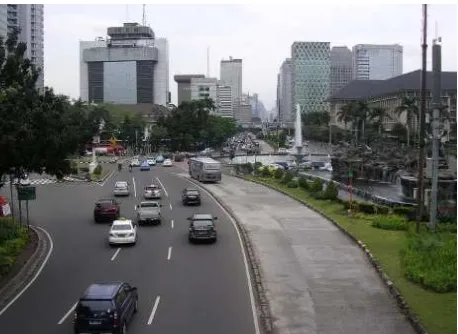
In this paper, the considered intersection consists of four-legs intersection located in Central Jakarta. The intersection is the meeting point of the four main roads, which from the north is Medan Merdeka Barat street (leg 1), from the west is Budi Kemulyaan street (leg 2), from the south is M.H. Thamrin street (leg 3), and from the east is Medan Merdeka Selatan street (leg 4). This intersection is shown in Figure 1.
2. Queue Length Vehicles Model
In this paper, the queue length of vehicles is the considered parameter to measure traffic congestion.
The queue length of vehicles in leg 1 and leg 3 after one cycle is shown in equation 1. The queue length of vehicles in leg 2 and leg 4 after one cycle is shown in equation 2.
� = �0+ (� − �)��+ ��� (1)
� = �0 + ���+ (� − �)�� (2)
where Q is a queue length of vehicles after one cycle, Q0 is a queue length of vehicles at the beginning of cycle. λ is the number of vehicles entering each leg intersection per second. μ is the number of vehicles going out of each leg intersection per second.
Figure 1. Intersection of Medan Merdeka Barat street, Budi Kemulyaan street, M.H. Thamrin street, and Medan Merdeka
Selatan street.
2015 International Conference on Automation, Cognitive Science, Optics, Micro Electro-Mechanical System, and Information Technology (ICACOMIT), Bandung, Indonesia, October 29–30, 2015
Green time (Tg) is the length of time of the green phase for leg 1 and leg 3, and also the length of time of the red phase for leg 2 and leg 4. Red time (Tr) is the length of time of the red phase for leg 1 and leg 3, and also the length of time of the green phase for leg 2 and leg 4. Tn is the cycle time. In the calculation, the length of time of the yellow phase is included in the green phase. This is because of in the yellow phase the vehicle is allowed to get out of the leg intersection, like the condition of the green phase.
3. Data Collection
At each intersection leg, it was installed a video type vehicle detector. Data are collected on Saturday. To further focus of this paper, the data used in the analysis was the data between 17:00 PM to 18:00 PM. The data obtained from the vehicle detectors represents the number of vehicles coming out from the junction leg when the phase is green. To get the number of vehicles coming out of the leg intersection per second (μ), it is calculated from data on the number of vehicles coming out of the leg junction (Nk) divided by the length of time of the green phase (Tg) for each period. Value of the green time (Tg) for each period is known from existing traffic control system.
Vehicle detectors only knew the number of vehicles that coming out of the leg intersection, not the number of vehicles entering. Therefore, the number of vehicles entering the leg intersection per second (λ) is obtained by using data from other intersection which is the data taken from the number of vehicles coming out from the other intersection then entering one of the leg of the main intersections. The intersection is M.H. Thamrin street and Kebun Sirih street located next to the main intersection. As these intersections are connected by M.H. Thamrin street, the variable λ for leg 3 can be calculated. Due to limitations of the measurement data, the value of variable λ for leg 1, leg 2, and leg 4 are obtained by performing simulations based on the Poisson distribution.
To simulate events of the vehicles arrival based on the Poisson distribution, SimEvents features was used. SimEvents is a simulation tool in MATLAB software. Programming using SimEvents is by writing in the form of blocks connected in accordance with their respective functions. The program begins with the Event-Based Random Number block. This block is used to generate signals based on the distribution that user choose, which is the Poisson distribution. Signal output from the block is then transferred in table form by using Discrete Event Signal to Workspace block. In addition, the signal can also be seen in graphical
form by using the Signal Scope block. Simulations were performed for one hour interval.
The results of the simulation using SimEvents were the number of vehicles coming in every second during the simulated time interval. By adding the vehicles coming in the cycle time interval and divided by the cycle time for each period, the number of vehicles entering the leg intersection per second (λ) is obtained.
4. Calculation of Queue Length
Vahicles Based on Data
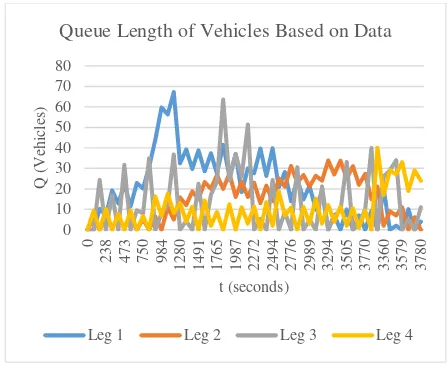
Based on the data from the vehicle detector, green time (Tg), red time (Tr), and cycle time (Tn), the queue length of vehicles can be calculated by using the equation 1 and the equation 2. Graph of the queue length of vehicles for each intersection leg is shown in Figure 2.
Figure 2. Queue length of vehicles based on data.
5. Queue Length Optimization of
Vehicles
The purpose of the paper is to design traffic signal control strategies at the road intersection. Optimization was done in order to generate optimal traffic signal. The parameter used to measure the level of congestion is a queue length of vehicles. The lowest level of traffic congestion is represented by the smallest value of the parameter [3]. In this case, the intersection with four legs is considered. Therefore, the objective function is selected as the total number of queue length of vehicles on each intersection leg.
The traffic signal is controlled based on the data traffic in the field. The green time (Tg) and the red time (Tr) are determined based on the queue length of vehicles of each intersection leg, in order to produce a minimum total queue length of vehicles
0
Queue Length of Vehicles Based on Data
of the four-legs intersection. The cycle time of each period is kept constant. Because this system is controlled in two phase system settings, then the variable red time (Tr) can be replaced by cycle time (Tn) minus variable green time (Tg). This makes the variables that need to be searched is reduced to only green time (Tg).
The larger green time (Tg) will cause queue length of vehicles on leg 1 and leg 3 are getting smaller. However, it can also cause a red time (Tr) becomes smaller, so queue length of vehicles on the leg 2 and leg 4 becomes larger. Therefore, it is of interest to perform optimization in order to find the value of the optimal green time (Tg) so that the resulting total length of the queue of vehicles (QTotal) is minimum. The minimum total lenght is defined by equation 3.
The cycle time for each period is held constant, which is 140 seconds. Green time (Tg) cannot have negative value and cannot be more than the cycle time. To give a red signal at least 5 seconds for each phase in each period, then the green signal (Tg) is limited to 5 seconds to 135 seconds. Limitation green signal (Tg) is defined by a constraint in the equation 3. The problem is fowmulated as:
min� �� Matlab which is used in solving the optimization problem to find the minimum value of a function with one variable in a fixed interval. This function searches the minimum value of a function by using parabolic interpolation technique.
6. Results and Analysis
Each period has a different value of λ and μ, so the optimal value of green signal (Tg) is different for each period. In addition, the queue length of vehicles at the beginning of each period will also affect the optimal value of green time (Tg). In Figure 3, it is shown the optimal value of green time (Tg) for each period.
The average value of λ for leg 1 is based on the data is 0.20 vehicle/s. The average value of λ for leg 2 is 0.06 vehicle/s. The average value of λ for leg 3 is 0.37 vehicle/s. The average value of λ to leg 4 is 0.10 vehicle/s. The average value of μ based on data for leg 1 was 0.30 the vehicle/s. Meanwhile, the average value of μ for leg 2 is 0.21 vehicle/s. The average value of μ for leg 3 is 0.61
vehicle/s. The average value of μ to leg 4 is 0.33 vehicle/s.
Figure 3. Optimal value of green time (Tg) for each cycle in 140 seconds cycle time.
Referring to the flow rate data of the number of vehicles entering the intersection (λ), it was known that the optimal value of the green time (Tg) was proportionally to the number of vehicles entering the intersection (λ). This condition was required in order to accommodate the large number of vehicles entering the intersections, such that the number of vehicles that came out can also be much more.
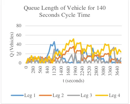
Based on the result of the optimal green time (Tg), then the queue length of vehicles (Q) for each leg intersection can be calculated by using equation 1 and equation 2. The result queue length of vehicles (Q) for each leg intersection with cycle time 140 seconds is shown in Figure 4.
Figure 4. Queue length of vehicles for 140 seconds cycle time.
Figure 4 shows the queue length of vehicle on each intersection leg were increasing and decreasing. This is due to the presence of the red phase and green phase in order to control the traffic at the intersection. When the red phase, the vehicles must stop and cause the increase of the queue length. Meanwhile, when the green phase, the vehicles are
0
The Optimal Value of Green Time (Tg) for Each Cycle.
Queue Length of Vehicle for 140 Seconds Cycle Time
allowed to run, so the queue length decreases. However, in green phase, the queue length can also increase. This possibility arises of how many vehicles that come to the intersection leg and how many vehicles that coming out during the green phase. The rate of the number of vehicles coming into the one of intersection leg is represented by the value of λ and the rate of the number of vehicles coming out from the intersection leg is represented by the value of μ.
To decrease the queue length of vehicles on a road, the number of vehicles coming (λ) must be smaller than the number of vehicles that exit (μ) of the road. If the number of vehicles coming (λ) is greater than the number of vehicles that exit (μ), then the queue length of vehicles is increased.
Optimization is performed to find the optimal green time value (Tg), so resulting the minimum of the queue length vehicle (Q) with a constant cycle time (Tn). Because the cycle time (Tn) is constant, then the variables that need to be searched is only green time (Tg). Red time (Tr) can be counted from the cycle time (Tn) minus green time (Tg).
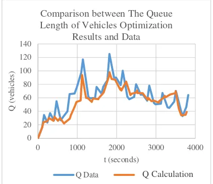
Figure 5. Comparison between the queue length of vehicles optimization results with 140 seconds cycle time and data.
Comparison of the queue length of vehicles optimization results for the 140 seconds cycle time compared to the queue length of vehicles based on field data gives the queue length of vehicles optimization results are smaller. Although, several queue lengths are bigger than the queue length data. Overall, the resulted total queue length of vehicles is smaller than the total queue length of vehicles based on the data as shown in Figure 5. The total queue length of the vehicle based on optimization results can reduce 10% of the total queue length of vehicles based on the data.
The average value of the optimal green time (Tg) is 100.037 seconds. The average value of the green
time (Tg) is bigger than the average value of the optimal red time (Tr). This is due to the largest value of the average rate of the number of vehicles coming (λ) is at the leg 3, so green phase given larger for leg 3. The increase and decrease in queue length of vehicles during the green phase is caused by the total vehicles coming (λ) and going out (μ) of each leg of the junction.
Figure 6. Comparison of total queue length of vehicles between different cycle time.
It was also calculated variation of cycle times, such as: 130 seconds, 150 seconds, 160 seconds, and 170 seconds. Calculations were performed using the same way as the calculation for cycle time 140 seconds. In Figure 6, it is shown a comparison of total queue length of vehicles between different cycle times.
Based on Figure 6, the result of the queue length of 140 seconds cycle time is the smallest compared to result queue length of other cycle times. Larger cycle time will make the red time increases. Hence, more vehicles have to stop at the intersection and the queue length gets bigger. For smaller cycle times, the green time is also becoming smaller. The vehicle can exit the intersection leg, then resulting in the accumulation of vehicles and queue length of vehicles get bigger too.
Based on the comparison of the queue length of vehicles on calculations for 140 seconds cycle time with the queue length of vehicles were based on the data, it is known that the queue length of vehicles on leg 1 was reduced by 49 %, queue length of vehicles on the leg 2 is reduced by 26 %, queue length of vehicles on the leg 3 was reduced by 41 %, while queue length of vehicles on the leg 4 increased up to 220 %. However, the total queue length of vehicles for 140 seconds cycle time results from this study can be reduced 10 % than the total queue length of vehicles based on the data. 0
0 1000 2000 3000 4000
Q
Comparison between The Queue Length of Vehicles Optimization
Results and Data
0 1000 2000 3000 4000
Q
Comparison of Total Queue Length of Vehicles Between Different Cycle
Time
Q 130 Q 140 Q 150
Q 160 Q 170
7. Conclusion
The paper presented the optimization of queue length of vehicles at road intersection. The optimization was solved by using the parabolic interpolation method to reduce the congestion that occurs at the road intersection. Results showed that the calculation with a cycle time of 140 seconds resulted the smallest total queue length of vehicles based on a comparison of the total queue length of vehicles between different cycle times, such that 130 seconds, 140 seconds, 150 seconds, 160 seconds, and 170 seconds
References
[1] Wootton, J.R., and Garcia-Ortiz, A. (1995) : Intelligent Transportation Systems: A Global Perspective, Mathematical and Computer Modelling, 22, 259-268.
[2] Morichi, S. (2005) : Long Term Strategy for Transport System in Asian Megacities, Journal of the 6th Eastern Asia Society for Transportation Studies International Conference in Bangkok, Thailand, 1-22.
[3] Bellemans, T., De Schutter, B., and De Moor, B. (2002) : Models for Traffic Control, Journal A, 43, 3-4, 13-22.
[4] Sakakibara, H., Aoki, M., and Matsumoto, H. (2005) : Advanced Traffic Signal Control System Installed in Phuket City, Kingdom of Thailand, SEI Technical Review June 2005, 60, 54-58.
[5] Sutandi, C. (2008) : Comparative Analysis of Advanced and Fixed Time Traffic Control System in Increasing Traffic Performance, Media Teknik Sipil Januari 2008, 51-58. [6] Golembiewski, G.A., and Chandler, B.
(2011) : Intersection Safety: A Manual for Local Rural Road Owners, US Department of Transportation, FHWA-SA-11-08.
[7] Underwood, R.T. (1991) : The Geometric Design of Roads, Macmillan Company of Australia: Australia.
[8] Robinson, B, etc. (2000) : Roundabouts: An Informational Guide. US Department of Transportation, FHWA-RD-00-067.
[9] Koonce, Peter, etc. (2008) : Traffic Signal Timing Manual, US Department of Transportation, FHWA-HOP-08-024.
[10] Jabari, S.E., and Liu, H.X. (2012) : A Stochastic Model for Traffic Flow. Transportation Research Part B, 46, 156-174. [11] Yates, R.D., and Goodman, D.J. (2005) :
Probability and Stochastic Processes A Friendly Introduction for Electrical and Computer Engineers Second Edition. John Wiley & Sons, Inc: USA.
[12] Ross, S. (2009): Introduction to Probability and Statistics for Engineers and Scientist Fourth Edition, Elsevier, Inc: Canada.
[13] Clune, M.I., and Cassandras, C.G. (2006) : Discrete Event and Hybrid System Simulation with SimEvents Discrete Event Systems 8th, International Workshop, 386-387.