DOES TOPOGRAPHIC NORMALIZATION OF LANDSAT IMAGES IMPROVE
FRACTIONAL TREE COVER MAPPING IN TROPICAL MOUNTAINS?
H. Adhikari a, *, J. Heiskanen a, E. E. Maeda a, P. K. E. Pellikka a
a University of Helsinki, Department of Geosciences and Geography, P.O. Box 68, FI-00014, Helsinki, Finland – (hari.adhikari, janne.heiskanen, eduardo.maeda, petri.pellikka)@helsinki.fi
KEY WORDS: Landsat, Fractional tree cover, Topographic correction, Digital Elevation Model, LiDAR
ABSTRACT:
Fractional tree cover (Fcover) is an important biophysical variable for measuring forest degradation and characterizing land cover. Recently, atmospherically corrected Landsat data have become available, providing opportunities for high-resolution mapping of forest attributes at global-scale. However, topographic correction is a pre-processing step that remains to be addressed. While several methods have been introduced for topographic correction, it is uncertain whether Fcover models based on vegetation indices are sensitive to topographic effects. Our objective was to assess the effect of topographic correction on the accuracy of Fcover modelling. The study area was located in the Eastern Arc Mountains of Kenya. We used C-correction as a digital elevation model (DEM) based correction method. We examined if predictive models based on normalized difference vegetation index (NDVI), reduced simple ratio (RSR) and tasseled cap indices (Brightness, Greenness and Wetness) are improved if using topographically corrected data. Furthermore, we evaluated how the results depend on the DEM by correcting images using available global DEM (ASTER GDEM, SRTM) and a regional DEM. Reference Fcover was obtained from wall-to-wall airborne LiDAR data. Landsat images corresponding to minimum and maximum sun elevation were analyzed. We observed that topographic correction could only improve models based on Brightness and had very small effect on the other models. Cosine of the solar incidence angle (cos i) derived from SRTM DEM showed stronger relationship with spectral bands than other DEMs. In conclusion, our results suggest that, in tropical mountains, predictive models based on common vegetation indices are not sensitive to topographic effects.
1. INTRODUCTION
Landsat satellite images became available for free in 2008, which together with systematic data acquisition plan has fortified Landsat’s role as a primary source of information for global land change research (e.g., Wulder et al., 2012). Landsat images also have good data consistency among Landsat missions and historical archive since 1972. The pre-processing methods of Landsat data have reached the level of maturity and pre-processed data sets have become available (e.g. Landsat Climate Data Record (CDR)) similar to moderate resolution data e.g. various MODIS data products (Masek et al., 2006). However, topographic correction remains as one of the pre-processing steps that have not been addressed globally.
Topographical effects in satellite images are caused by illumination differences between the sunlit and shaded slopes. The magnitude of the effect depends on the time of the year because of variations in the sun elevation. Hence, in the topographic normalization, the dependency of reflectance factors on topographic position is removed. Topographic correction has been shown to improve land cover mapping using object-based classification (Moreira & Valeriano, 2014) and land cover classification accuracy (Pellikka, 1996; Vanonckelen et al., 2013).
Topographic correction methods can be grouped into three categories: those based on band ratios, those based on a Hyperspherical Direction Cosine Transformation (HSDC), and those requiring digital elevation model (DEM). DEM-based methods, can be summarized as three broad types: (1) empirical methods, (2) Lambertian methods and (3) non-Lambertian methods (Gao & Zhang, 2009). The most often used methods are
* Corresponding author.
Lambert cosine correction (Meyer et al., 1993), Minnaert correction (Smith et al., 1980), C-correction (Teillet et al., 1982) and Sun-canopy-sensor method (Gu & Gillespie, 1998). Several studies have demonstrated the viability of C-correction for radiometric correction of multitemporal images taken under different illumination conditions (Moreira & Valeriano, 2014; Reese & Olsson, 2011; Vanonckelen et al., 2013).
Continuous fields of vegetation attributes can be estimated using a multitude of predictors derived from Landsat images. However, the topographic effect on different types of predictors can be different. For example, canopy cover, fractional tree cover (Fcover) and leaf area index (LAI) are typically estimated based on vegetation indices such as Normalized Difference Vegetation Index (NDVI) and Reduced Simple Ratio (RSR) (Majd et al., 2013; Korhonen et al., 2013; Wu, 2011).
NDVI is a simple index used to accentuate vegetation from imagery containing reflectance in the red and NIR portions of the spectrum. RSR is an empirical SWIR modification to the simple ratio (SR) vegetation index (Brown et al., 2000). Both indices attempt to depress background reflectance and improve the accuracy in extracting vegetation information from remotely sensed data.
Tasseled Cap transformation (TC) compress spectral data into bands associated with the physical characteristics of scene (Crist, 1985). TC indices (Brightness, Greenness and Wetness) have been used, for example, for forest disturbance detection (Healey et al., 2005; Jin & Sader 2005; Skakun et al. 2003) and forest classification (Dymond et al., 2002).
topography requires a DEM. Currently, there are several sources of global DEMs, such as SRTM and ASTER DEM. SRTM DEM at 30 m resolution was made recently globally available (https://lta.cr.usgs.gov/SRTM1Arc), improving its applicability for topographic correction of Landsat data. In addition to the global DEMs, many areas are supplemented by regional DEMs based on topographic map data. However, viability of different DEMs for topographic correction have been rarely assessed.
Several authors have compared topographic correction methods for Landsat data (e.g., Hantson & Chuvieco, 2011; Moreira & topographic correction improves the accuracy of continuous variables (Törmä & Härmä, 2003), such as Fcover. Furthermore, classification is typically based on individual bands, but not vegetation indices, which are commonly used in Fcover, LAI and biomass mapping.
In this study, our objective was to assess the effect of topographic correction on the accuracy of Fcover predictions based on Landsat images with and without topographic correction. In particular, we aimed to examine if predictive models based on NDVI, RSR and TC indices are affected differently, and if results depend on the source of DEM.
2. MATERIAL AND METHODS
2.1 Study area
The Taita Hills (3°25´S, 38°20´E) are located in the northernmost part of the Eastern Arc Mountains in southeastern Kenya (Figure 1). The area is characterized by distinct topographical variation and the mountainous hills raise up to 2200 m a.s.l. from the Tsavo Plains at 600−900 m a.s.l. Taita Hills are considered as one of the world’s most important biodiversity hotspots. However, due to the favorable climate and edaphic conditions, the indigenous cloud forests of the Taita Hills have suffered substantial deforestation and degradation due to agriculture, grazing and logging of forest for firewood and charcoal manufacturing since the early 1960´s (Pellikka et al., 2009).
2.2 Landsat images
Landsat surface reflectance (CDR) is a product of the Landsat Ecosystem Disturbance Adaptive Processing System (LEDAPS) at the National Aeronautics and Space Administration (NASA) Goddard Space Flight Center. The images have been calibrated to radiance, converted to top-of-atmosphere reflectance and then atmospherically corrected using the MODIS/6S methodology (Masek et al., 2006).
The Taita Hills lies on the south east quarter of the Landsat image (WRS path 167 and row 62). Landsat scenes with cloud cover
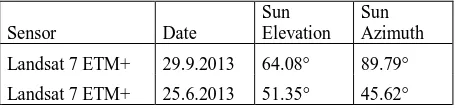
less than 30% in the lower right quarter in 2013 were downloaded and two images less affected by cloud, shadow and missing data due to Scan line corrector (SLC) off and corresponding to the minimum and maximum sun elevation were used in this study. Both images were acquired at 7:32 UTC time in the morning and image processing level was L1T.
2.3 Digital elevation models
DEM used for topographic correction were obtained from various sources. Advanced Spaceborne Thermal Emission and Reflection Radiometer (ASTER) Global Digital Elevation Model (GDEM) has been generated from the stereoscopic ASTER satellite images. ASTER GDEM is available at the resolution of 30 m. The ASTER GDEM covers land surfaces between 83°N and 83°S. It is a product of Ministry of Economy, Trade, and Industry (METI) and the National Aeronautics and Space Administration (NASA) (https://www.jspacesystems.or.jp/ersdac/GDEM/E/4.html).
Shuttle Radar Topography Mission (SRTM) 1 arc-second global elevation data has been available since 23 September 2014 (https://lta.cr.usgs.gov/SRTM1Arc). SRTM provides DEM for 80% of the earth’s surface (all land areas between 60° N and 56° S). SRTM is a joint project between the National Geospatial-Intelligence Agency (NGA) and NASA. The DEM has been filled to remove small artifacts.
All Landsat images, ASTER and SRTM DEM were downloaded from the United States Geological Survey (USGS) Earth Explorer platform (http://earthexplorer.usgs.gov/).
A regional DEM (TOPO DEM) for the Taita Hills was created using the contour lines of the topographic maps at 1:50 000 scale produced by the Survey of Kenya (Pellikka et al., 2004). DEM has a pixel size of 20 m × 20 m, and it was resampled to 30 m × 30 m pixel size similar to the Landsat images.
2.4 Airborne LiDAR data and fractional tree cover
We used Fcover (1–canopy gap fraction) derived from airborne LiDAR as a reference data. Previous studies have shown that LiDAR provides canopy cover and gap fraction estimates with an accuracy comparable to the field measurements (Korhonen et al., 2011; Heiskanen et al., in press). Furthermore, wall-to-wall LiDAR data provided a large sample size and the use of random sampling scheme in the logistically difficult terrain.
Sensor Date
Table 1. Details of Landsat images used in this study.
Figure 1. Location of the study area and hillshade view of the topography.
The discrete return LiDAR data was acquired 4–5 February 2013 for 10 km × 10 km area (Table 2). Data were pre-processed by the data vendor (Topscan Gmbh) and delivered as georeferenced point cloud in UTM/WGS84 coordinate system with ellipsoidal heights. Vendor also filtered ground returns by using Terrascan software (Terrasolid Oy). Furthermore, we filtered buildings and powerlines. Then, the ground returns were used to generate DEM at 1 m cell size. We also removed the overlap between the adjacent flight lines based on minimum scan angle using lasoverage tool in LAStools software (rapidlasso GmbH).
FUSION software (McGaughey, 2014) was used for computing a proxy of Fcover. We extracted LiDAR returns for 90 m × 90 m sample plots corresponding to 3 × 3 pixel windows of Landsat ETM+ images. Heiskanen et al. (in press) found that all echo cover index (ACI) (e.g., Morsdorf et al., 2006) gave an unbiased estimate of canopy gap fraction using the same LiDAR data. Hence, we used ACI as a proxy of Fcover. ACI was computed as:
ACI (%) = ∑Allcanopy
∑All (1)
where, All refers to the returns of all return types (i.e. single, first, intermediate and last returns) and canopy refers to the returns
from the forest canopy. Laser returns with height less than 1.5 m from the ground were considered as ground in order to exclude understory vegetation from Fcover.
2.5 Topographic correction of Landsat-data
C-correction is a semi-empirical topographic correction method, which consists of a modified cosine correction with the empirical parameter cλ (Reese & Olsson, 2011). cλ (Eq. 4) is calculated for every band (λ) separately based on the linear relationship (Eq. 3) between the spectral data and the cosine of the solar incidence angle (cos i) (Eq. 2). Each band were topographically corrected using Eq. 5.
cos � = cos �� × cos � + �� �� × �� � × � � − � (2)
ρλ, = λ+ λ× cos�
(3)
λ=�λλ
(4)
ρλ, = ρλ, c ��+ �
c � + � (5)
where,
i = solar incidence angle with respect to surface normal sz = solar zenith angle
sl = slope
az = solar azimuth angle as = aspect
ρλ,t = topographically influenced (t) reflectance of band λ bλ = intercept of linear regression
mλ = slope of linear regression
cλ = c-factor calculated for every band separately
ρλ,n = topographically normalized (n) reflectance of band λ
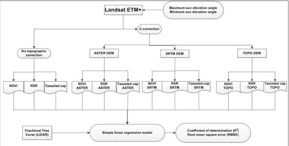
cos i, slope and aspect were calculated from each DEM. Resolution of each DEM was made similar to Landsat image. Areas with a slope ≤ 2% were not included in the parameter estimation. Land cover stratification based on NDVI has been successfully used to consider the land cover dependency of cλ Figure 2. Overview of the methodology
Parameter Value
Date of acquisition 4–5 February, 2013
Sensor Optech ALTM
Mean flying height (m AGL) 760
Flying speed (knots) 116–126
Pulse rate (kHz) 100
Scan rate (Hz) 36
Maximum scan angle (degrees) 16 Pulse density (pulses m−2) 9.6 Return density (returns m−2) 11.4 Maximum number of returns per pulse 4 Beam divergence at 1/e2 (mrad) 0.3
Footprint diameter (cm) 23
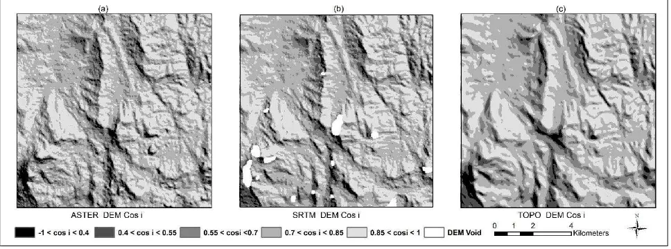
(Hantson & Chuvieco, 2011; McDonald et al., 2000). The study area was divided into three NDVI classes. Class 1 (NDVI < 0.4) covered urban areas, bare areas, grasslands and agriculture lands, Class 2 (NDVI 0.40.6) covered secondary forest, plantation and regeneration and Class 3 (NDVI 0.61) covered indigenous forest. Each class was further subdivided into five sub classes (-1−0.4, 0.4–0.55, 0.55−0.70, 0.70–0.85, 0.85−1.0) based on cos i (Figure 3). 500 samples from each sub class, i.e. 2500 samples for each class and 7500 samples for each image were selected for linear regression between cos i and spectral bands. cλ was calculated for each NDVI class and each band.
2.6 Predictor variables for fractional tree cover
NDVI, RSR and TC indices (Brightness, Greenness and Wetness) were used as predictor variables. NDVI combines information only from NIR and Red bands, but RSR includes additional SWIR bands to reduce the effects of background reflectance (Brown et al., 2000). Since Landsat ETM+ images were in surface reflectance, tasseled cap coefficients for Landsat TM reflectance factor data were used.
NDVI
=
((NIRNIR+-RR)) (6)RSR =
NIRR×
(SWIR maxSWIR max-SWIR min)-SWIR(7)
Brightness = 0.2043 × B + 0.4158 × G + 0.5524 × R + 0.5741 × NIR + 0.3124 × SWIR1 + 0.2303 × SWIR2 (8)
Greenness = -0.1603 × B - 0.2819 × G - 0.4934 × R + 0.7940 × NIR - 0.0002 × SWIR1 - 0.1446 × SWIR2 (9)
Wetness = 0.0315 × B + 0.2021 × G + 0.3102 × R + 0.1594 × NIR - 0.6806 × SWIR1 - 0.6109 × SWIR2 (10) where, B =blue band (450−520 nm), G = green band (520−600 nm), R= red band (630−690 nm), NIR= NIR band (770−900 nm), SWIR1=SWIR band (1550−1750 nm) and SWIR2= SWIR band (2090−2350 nm). SWIR1max and SWIR1min were defined as 99% and 1% points in the cumulative histogram of the SWIR1 respectively. NDVI, RSR and TC indices were calculated from topographically corrected and non-topographically corrected surface reflectance values of Landsat ETM + spectral bands.
Finally, 2000 random sample plots (size of 90 m × 90 m corresponding to 3 pixels × 3 pixels windows of Landsat image) were chosen for extracting average NDVI, RSR, Brightness, Greenness and Wetness from Landsat image and for computing Fcover from LiDAR data. Only sample plots without any missing data were retained for the further analysis. Hence, the number of sample plots was reduced to around 1500.
2.7 Regression analysis
We used simple linear regression to model relationships between Fcover and NDVI, RSR, and TC indices. The results were evaluated based on coefficient of determination (R2) and root mean square error (RMSE).
3. RESULTS
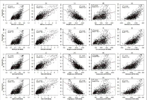
The various predictor variables explained variation in Fcover differently (Figure 4). Out of all predictors, the highest R2 and the lowest RMSE were obtained using RSR. NDVI and Greenness showed the weakest relationships with Fcover. NDVI, RSR, Greenness and Wetness showed positive correlation with Fcover as they are affected by the amount of vegetation, while Brightness had negative correlation as it increases with the higher amount of open soil and lower vegetation cover.
The strength of the relationship also varied between the images acquired under different illumination conditions (Table 3). NDVI, RSR, Brightness, Greenness and Wetness explained more variation in Fcover when extracted from the image with higher sun elevation angle (29.9.2013). For example, topographically uncorrected Brightness indices explained only 37.5% of variation in Fcover when extracted from the lower sun elevation angle image in comparison to 45.2% when extracted from the higher sun elevation angle image. NDVI was also affected by the time of image acquisition. This was consistent for all the predictor variables.
The effect of topographic correction on Fcover regression models was not consistent for all predictors (Figure 4 and Table 3). The models based on Brightness and Wetness showed some improvement in terms of R2 and RMSE but other models were not significantly affected, particularly when based on the larger solar elevation angle image. In the case of NDVI, there was no improvement at all due to topographic correction in either image. Figure 3. Five cos i classes based on (a) ASTER DEM, (b) SRTM DEM and (c) TOPO DEM.
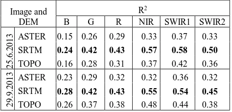
The source of DEM also affected the results in different ways (Figure 4, Table 3), although differences were small like improvements in the model fit due to topographic correction. However, SRTM DEM performed better for Brightness and Greenness indices which were most affected by the topographic correction. Furthermore, when estimating c-factors by regression, the relationships between cos i and spectral bands were the strongest in terms of R2 (Table 4) when derived from SRTM DEM.
4. DISCUSSION
According to our result RSR had the strongest linear relationship with Fcover obtained from LiDAR data. NDVI showed weak relationship with Fcover. These results are similar to those obtained by Korhonen et al. (2013) from a boreal forest site. However, our results differ from Majd et al. (2013) and Wu (2011) who found strong relationship between Fcover and NDVI in pecan orchards and savannas ecosystem. Weak relationship between NDVI and Fcover can be explained by the heterogeneous landscape in the study area and saturation of NDVI as the study area contains also patches of mountain rain forests.
However, it is difficult to say if this is due to weaker topographic effects or a result of variations in vegetation phenology. Image with lower sun elevation match better in terms of phenology to LiDAR acquisition.
Furthermore, our results demonstrate that topographic correction has very small or no effect on Fcover models. In the case of NDVI, no improvement was observed. Therefore, topographic correction might not be necessary for achieving the best Fcover prediction accuracy in tropical mountains that have relatively high solar elevation angles. In particular, models based on ratio based vegetation indices seem to be not affected by topographic correction. The fact that NDVI is less sensitive to topographic conditions has also been demonstrated by Matsushita et al. (2007). However, with multiplicative indices (e.g. Brightness), topographic correction is likely to have considerable effect.
Even though artifacts could be clearly observed in the SRTM DEM, it performed well in comparison to other sources of DEM, in agreement with similar previous studies (Vanonckelen et al., 2013; Balthazar et al., 2012). Most noticeably, SRTM DEM provided better R2 in the C-correction than regional DEM based on the best topographic maps of the study area.
needed across larger latitudinal range because topographic effects increase with increasing latitude and decreasing solar elevations.
5. CONCLUSIONS
We assessed the effect of topographic correction on the accuracy of Fcover predictions based on Landsat images. Several sources of DEM were evaluated when performing the topographic correction. Among the tested indices, RSR provided the best regression model for Fcover. There were no major difference between the linear models based on topographically corrected or non-corrected NDVI and RSR, which indicates that NDVI and RSR are relatively robust against topographical effects. Therefore, in tropical mountain environments, studies based on NDVI or RSR do not necessarily need to consider the effect of topography. However, topographic correction should be considered for lower sun elevation angle images if models are developed using TC Brightness or Wetness. Finally, SRTM was
shown to be the best DEM source for topographic corrections in the tested conditions.
ACKNOWLEDGEMENTS
The authors acknowledge Building Biocarbon and Rural Development in West Africa (BIODEV) project funded by the Ministry for Foreign Affairs of Finland. Mr. Adhikari holds a grant from CIMO of Finland (Center for International Mobility). Dr. Eduardo Maeda is currently funded by a research grant from the Academy of Finland.
REFERENCES
Balthazar, V., Vanacker, V., & Lambin, E. F., 2012. Evaluation and parameterization of ATCOR3 topographic correction method for forest cover mapping in mountain areas. Int. J. Appl. Earth Obs. Geoinf. (18), pp. 436–450.
Brown, L., Chen, J. M., Leblanc, S. G., & Cihlar, J., 2000. A shortwave infrared modification to the simple ratio for LAI retrieval in boreal forests: An image and model analysis. Remote Sens. Environ., 41 (1), pp.16-25.
Crist, E. P., 1985. A TM tasseled cap equivalent transformation for reflectance factor data. Remote Sens. Environ., 17, pp. 301-306.
Dymond, C.C., Mladenoff, D.J., & Radeloff, V.C., 2002. Phenological differences in Tasseled Cap indices improve deciduous forest classification. Remote Sens. Environ., 80, pp. 460-472.
Gao, Y.N., & Zhang, W.C., 2009. A simple empirical topographic correction method for ETM+ imagery. Int. J. Remote Sens., 30 (9), pp. 2259–2275.
Gu, D., & Gillespie, A., 1998. Topographic normalization of Landsat TM images of forest based on subpixel sun-canopy-sensor geometry. Remote Sens. Environ., 64, pp. 166-175.
Hantson, S., & Chuvieco, E., 2011. Evaluation of different topographic correction methods for Landsat imagery. Int. J. Appl. Earth Obs. Geoinf., 13, pp. 691-700.
Healey, S.P., Cohen, W.B., Zhiqiang, Y., & Krankina, O.N., 2005. Comparison of Tasseled Cap-based Landsat data structures for use in forest disturbance detection. Remote Sens. Environ., 97, pp. 301-310.
Heiskanen, J., Korhonen, L., Hietanen, J., Pellikka, P. K. E., in press. Airborne LiDAR for estimating canopy gap fraction and leaf area index of tropical montane forests. Int. J. Remote Sens.
Jin, S., & Sader, S.A., 2005. Comparison of time series tasseled cap wetness and the normalized difference moisture index in detecting forest disturbances. Remote Sens. Environ., 94, pp. 364-372.
Korhonen, L., Korpela, I., Heiskanen, J., Maltamo, M., 2011. Airborne discrete-return LiDAR data in the estimation of vertical canopy cover, angular canopy closure and leaf area index. Remote Sens. Environ. 115(4), pp. 1065-1080.
Predictor variables
Table 3. Summary of the linear regression results between different predictor variables and Fcover, and two images. The predictors with subscripts were topographically corrected using either ASTER, SRTM and TOPO DEM. Values in bold are the highest R2 and lowest RMSE. All the models were statistically highly significant (p < 0.0001).
Image and
Table 4. The mean R2 of three NDVI classes obtained from the linear regression between cos i from different DEMs and each spectral bands from the two images. Values in bold are the highest R2.
Korhonen, L., Heiskanen, J., & Korpela, I., 2013. Modelling lidar-derived boreal forest canopy cover with SPOT 4 HRVIR data. Int. J. Remote Sens., 34, pp. 8172-8181.
Majd A. M. S., Bleiweiss, M. P., DuBois, D., & Shukla, M. K., 2013. Estimation of the fractional canopy cover of pecan orchards using Landsat 5 satellite data, aerial imagery, and orchard floor photographs. Int. J. Remote Sens., 34(16), pp. 5937-5952.
Masek, J. G., Vermote, E. F., Saleous, N. E., Wolfe, R., Hall, F. G., Huemmrich, K. F., Gao, F., Kutler, J., & Lim, T. K., 2006. A Landsat Surface Reflectance Dataset for North America, 1990– 2000. IEEE Geosci. Remote. Sens. Let., 3(1). pp. 68-72.
Matsushita, B., Yang, W., Chen, J., Onda, Y., & Qiu, G., 2007. Sensitivity of the Enhanced Vegetation Index (EVI) and Normalized Difference Vegetation Index (NDVI) to Topographic Effects: A Case Study in High-Density Cypress Forest. Sensors 7, pp. 2636-2651.
McDonald, E.R., Wu, X., Caccetta, P.A., & Campbell, N.A., 2000. Illumination correction of Landsat TM data in south east NSW. Paper Presented at: Proceedings of the Tenth Australasian Remote Sensing Conference.
McGaughey, R. J., 2014. FUSION/LDV: Software for LIDAR Data Analysis and Visualization. United States Department of Agriculture, Forest Service, Pacific Northwest Research Station.
Meyer, P., Itten, K. I., Kellenberger, T., Sandmeier, S., & Sandmeier, R., 1993. Radiometric corrections of topographically induced effects on Landsat TM data in an alpine environment. ISPRS J. Photogramm. Remote, Sens., 484, pp. 17–28.
Moreira, E.P., & Valeriano, M.M., 2014. Application and evaluation of topographic correction methods to improve land cover mapping using object-based classification. Int. J. Appl. Earth Obs. Geoinf., 32, pp. 208-217.
Morsdorf, F., Kötz, B., Meier, E., Itten, K. I., Allgöwer, B., 2006. Estimation of LAI and fractional cover from small footprint airborne laser scanning data based on gap fraction. Remote Sens. Environ. 104(1), pp. 50-61.
Pellikka, P., 1996. Illumination compensation for aerial video image to improve land cover classification accuracy in the mountains. Can. J. Remote Sens. 22:4, pp. 368-381.
Pellikka, P., Clark, B., Hurskainen, P., Keskinen, A., Lanne, M., Masalin K., Nyman-Ghezelbash, P., & Sirviö, T., 2004. Land use change monitoring applying geographic information systems in the Taita Hills, SE-Kenya. In the Proceedings of the 5th African Association of Remote Sensing of Environment Conference, 17-22 Oct. 2004, Nairobi, Kenya.
Pellikka, P., Lötjönen, M., Siljander, M., & Lens, L., 2009. Airborne remote sensing of spatiotemporal change 1955-2004 in indigenous and exotic forest cover in the Taita Hills, Kenya. Int. J. Appl. Earth Obs. Geoinf., 11, pp. 221 -232.
Reese, H., & Olsson, H., 2011. C-correction of optical satellite data over alpine vegetation areas: A comparison of sampling strategies for determining the empirical c-parameter. Remote Sens. Environ., 115, pp. 1387–1400.
Skakun, R.S., Wulder, M.A., & Franklin, S.E., 2003. Sensitivity of the thematic mapper enhanced wetness difference index to detect mountain pine beetle red-attack damage. Remote Sens. Environ., 86, pp. 433-443.
Smith, J. A., Lin, T. L., & Ranson, K. J., 1980, The Lambertian assumption and Landsat data. Photogramm. Eng. Remote Sens., 46, pp.1183–1189.
Teillet, P. M., Guindon, B., & Goodenough, D. G., 1982. On the slope-aspect correction of multispectral scanner data. Can. J. Remote Sens. 8(2), pp. 84–106.
Törmä, M., & Härmä, P., 2003. Topographic correction of landsat ETM-images in Finnish Lapland. Geoscience and Remote Sensing Symposium, IGARSS '03. Proceedings. IEEE International, 6, pp. 3629-3631.
Vanonckelen, S., Lhermitte, S., & Van Rompaey, A., 2013. The effect of atmospheric and topographic correction methods on land cover classification accuracy. Int. J. Appl. Earth Obs. Geoinf., 24, pp. 9-21.
Wu, W., 2011. Derivation of tree canopy cover by multiscale remote sensing approach. ISPRS - Int. Arch. Photogramm. Remote Sens. Spa. Inf. Sci., XXXVIII-4 (W25), pp. 142-149.