APPLICATION OF SPATIAL MODELLING APPROACHES, SAMPLING STRATEGIES
AND 3S TECHNOLOGY WITHIN AN ECOLGOCIAL FRAMWORK
Hou-Chang Chena,Nan-Jang Lob, Wei-I Changc, andKai-Yi Huangd, *
a
Graduate student, Dept. of Forestry, Chung-Hsing University, Taiwan, R. O. C., E-mail: [email protected] b
Specialist, EPMO, Chung-Hsing University, Taiwan, R. O. C., E-mail: [email protected] c
Director, HsinChu FDO, Forest Bureau, Council of Agriculture, Taiwan R. O. C., E-mail: [email protected] d, *
Professor, Dept. of Forestry, Chung-Hsing University, Taiwan, R. O. C., E-mail: [email protected] 250 Kuo-Kuang Road, Taichung, Taiwan 402, R. O. C., Tel: +886-4-22854663; Fax: +886-4-22854663
Commission VIII/7
KEY WORDS: Modelling, Statistics, Experimental, Technology, Ecology, Forestry.
ABSTRACT:
How to effectively describe ecological patterns in nature over broader spatial scales and build a modeling ecological framework has become an important issue in ecological research. We test four modeling methods (MAXENT, DOMAIN, GLM and ANN) to predict the potential habitat of Schima superba (Chinese guger tree, CGT) with different spatial scale in the Huisun study area in Taiwan. Then we created three sampling design (from small to large scales) for model development and validation by different combinations of CGT samples from aforementioned three sites (Tong-Feng watershed, Yo-Shan Mountain, and Kuan-Dau watershed). These models combine points of known occurrence and topographic variables to infer CGT potential spatial distribution. Our assessment revealed that the method performance from highest to lowest was: MAXENT, DOMAIN, GLM and ANN on small spatial scale. The MAXENT and DOMAIN two models were the most capable for predicting the tree’s potential habitat. However, the outcome clearly indicated that the models merely based on topographic variables performed poorly on large spatial extrapolation from Tong-Feng to Kuan-Dau because the humidity and sun illumination of the two watersheds are affected by their microterrains and are quite different from each other. Thus, the models developed from topographic variables can only be applied within a limited geographical extent without a significant error. Future studies will attempt to use variables involving spectral information associated with species extracted from high spatial, spectral resolution remotely sensed data, especially hyperspectral image data, for building a model so that it can be applied on a large spatial scale.
1. NTRODUCTION
Building ecological modeling framework has been the core of ecological research since the latter half of the 20th century (Guisan and Zimmermann, 2000). It can provide a measure of a species’ occupancy potential in areas not covered by biological surveys and consequently is becoming an indispensable tool to conservation planning and forest management. Technological innovation over the last few decades, especially in the fields of remote sensing (RS) and geographic information systems (GIS), greatly enhanced scientists’ capacity to meet this challenge by giving them the ability to describe patterns in nature over broader spatial scales and at a greater level of detail than ever before (Guisan and Zimmermann, 2000). Besides, advances in statistical techniques enhance the ability of researchers to tease apart complex relationships, while effectively incorporated of RS and GIS tools permit more accurate descriptions of spatial patterns and suggest directions for species distribution. Several alternative methods have been used to predict the geographical distributions of species (Elith et al., 2006). We used maximum entropy (MAXENT), DOMAIN modeling (DOMAIN), generalized linear model (GLM) and artificial neural networks (ANN) to build model because they are easy to use and produce useful prediction in other research (Carpenter et al., 1993; Lek and Guegan, 1999; Guisan et al., 2002; Elith et al., 2006; Phillps et al., 2006; Phillps et al., 2008).
Despite the extensive use of species distribution models, some important conceptual, biotic and algorithmic uncertainties need to be clarified in order to improve predictive performance of
these models (Araújo and Guisan, 2006). For instance, species ecological characteristics, sample size, model selection and predictor contribution (Araújo and Guisan, 2006). Hence, it must be interpreted carefully of species’ occupancy potential in areas not covered by biological surveys. Generally, models for species with broad geographic ranges and environmental tolerance tend to be less accurate than those for species with smaller geographic ranges and limited environmental tolerance (Thuiller et al., 2004; Elith et al., 2006).
build predictive models. (5) The multi-modeling assessment approach was performed in this study. This included the application of a single model to data describing patterns at different spatial scales and the comparison of several models using a common dataset.
2. STUDY AREA
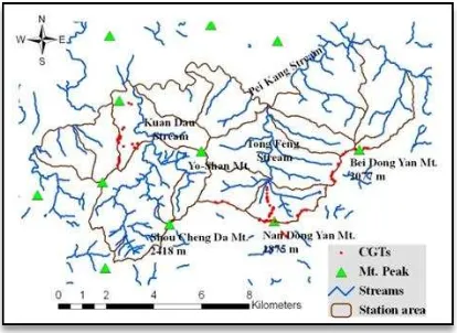
We chose a rectangular study area, encompassing the Huisun Forest Station, and it has a total area of 17,136 ha. The Huisun Forest Station is in central Taiwan, situated within 24◦2´–24◦5´ N latitude and 121◦3´–121◦7´ E longitude (Figure 1). This station is the property of National Chun-Hsing University. The entire study area ranges in elevation from 454 m to 3,418 m, and its climate is temperate and humid. In addition, the study area has nourished many different plant species more than 1,100 and is a representative forest in Taiwan. It comprises five watersheds,including two larger watersheds, Kuan-Dau at west and Tong-Feng at east. So far, all of the Chinese guger-tree samples (in situ data) were collected from the Tong-Feng, Yo-Shan, and Kuan-Dau sites in the Huisun study area by using a GPS.
Figure 1. Location map of the study area
3. MATERIALS AND METHOD
3.1 Species occurrence data
We collected in situ CGTs data by using a GPS linked with a laser range, and then performed a post-processed differential correction that makes them have an accuracy of sub-meters. The dataset was eventually converted into ArcView shapefile format for later use. So far, CGT samples were collected from Tong-Feng (122), Yo-Shan (8), and Kuan-Dau (64) sites in the Huisun study area, respectively. Pseudo-absences were generated for those models that required them (all except DOMAIN) by taking 500 samples randomly in study area. Three sampling designs (SD) were created for model development and validation through different combinations of CGT samples from aforementioned three sites (see figure 1).
SD-1: we randomly selected two-thirds of Tong-Feng dataset for building “Tong-Feng base model” and the remaining one-third of that dataset for model validation.
SD-2: we used the same base model built in SD-1 and only used samples taken from Yo-Shan about 0.5 km away from the Tong-Feng site to test the base model.
SD-3: we still used the same base model in SD-1 and only used samples taken from the Kuan-Dau site about 5 km away from Tong-Feng site to test the base model. Then we evaluated the spatial extrapolation ability of the four models.
3.2 Environmental data
We collected digital elevation model (DEM) of 5 m resolution, orthophoto base maps (1:10,000), and two-date SPOT images. DEM was acquired from the Aerial Survey Office, Forestry Bureau of the Council of Agriculture, Taiwan. To meet the requirements of the study, the DEM was interpolated into 5 5 m grid size, geo-referenced to the coordinate system, TWD67 (Taiwan Datum, spheroid: GRS67) and Transverse Mercator map projection over two-degree zone with the central meridian 121E. The two-date SPOT-5 images were acquired from Center for Space and Remote Sensing Research, National Central University (CSRSR, NCU), Taiwan (© SPOT Image Copyright 2004 and 2005, CSRSR, NCU). System calibration and geometric correction with level 2B were performed on the images, and then they were rectified to the TWD67 Transverse Mercator map projection and resampled to 5 m resolution to be consistent with the layers from DEM. We chose the two-date SPOT-5 images (07/10/2004 and 11/11/2005) because they have the best quality with the amount of clouds less than 10%.
Elevation, slope, and aspect were generated from DEM by ERDAS Imagine software module, and hill-shade data layer by ArcGIS spatial analyst module. The ridges and valleys in the study area were used together with DEM to generate terrain position layer. The main ridges and valleys over the study area were directly interpreted from the orthophoto base maps; these lines were then digitized to establish the data layer by using ARC/INFO software for later use. The data layer in a vector format was then converted into a new data layer in a raster format by ERDAS Imagine software module, and then combined with DEM to generate terrain position layer (Skidmore, 1990). Vegetation indices were derived from the two-date SPOT images, one in autumn (11/11/2005), the other in summer (07/10/2004), based on the concepts stated in Hoffer (1978), and is expressed in equation (1):
summer summer
autumn autumn
MIR NIR
MIR NIR
3.3 Model development
Predictive distribution models were formulated using the four different modeling algorithms. The modeling algorithms are briefly described below.
We implemented maxent entropy using version 3.3.3 of the free software developed by S. Phillips and colleagues (http://www.cs.princeton.edu/~schapire/maxent/). And other methods implemented ModEco by using version 1.0 of the free software (http://gis.ucmerced.edu/ModEco/).
1) MAXENT can make predictions or inferences from incomplete information (Phillips et al., 2006), and may remain effective from small sample sizes (Kumar and Stohlgren, 2009). The principle of MAXENT is based on the concepts of thermodynamic entropy, and then is used to describe the probability distribution in several domains, and Bayesian statistics is for exploring the probability distribution of each
pixel when the entropy reach the maximum that the state would be extremely close to uniform distribution. That is, MAXENT would find out the type of probability distribution that is most likely occurring in the general state. The formula for MAXENT is shown in following equation (2):
Z
2) DOMAIN derives a point-to-point similarity metric to assign a classification value to a potential site based on its proximity in environmental space to the most similar occurrence. The Gower metric (Gower, 1971) provides a suitable means of quantifying similarity between two sites. The distance of d between two points A and B in a Euclidean p dimensional space is defined as equation (3):
We define the complementary similarity measure RAB:
RAB = 1 - dAB
R is constrained between 0 and 1 for points within the ranges use in Equation 3,
We define SA, the maximum similarity between candidate point A and the set of known record sites Tj as equation (5):
By evaluating S for all grid points in a target area, a matrix of continuous varying similarity values is generated which are not probability estimates, but degrees of classification confidence (Carpenter et al., 1993).
3) GLM is a generalization of general linear models. General class of linear models are made up of three components: random, systematic, and link function. Random component identifies response variable E(Y) and its probability distribution. Systematic component identifies the set of predictor variables (X1,...,Xk). Link function identifies a function of the mean that is a linear function g(μ) of the predictor variables. The formula for GLM is shown in following equation (3):
k
β = regression coefficients X = predictor variable
By using a logit link function that transforms the scale of the response variable, being able to relax the distribution and constancy of variances assumptions that are commonly required by traditional linear models (McCullagh and Nedler, 1989). Consequently, the GLM model is particularly suitable for predicting species distributions, and has been proven to be successful in various ecological applications (Guisan et al., 2002).
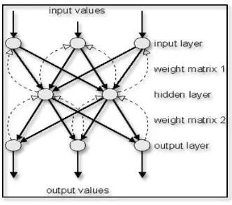
4) Back-propagation artificial neural network (BPANN) consists of input, hidden, and output layers. The input layer may contain information about individual training pixels including percent spectral reflectance in various bands and ancillary data such as elevation, slope, etc.
Each layer consists of nodes that are interconnected. This interconnectedness allows information to flow in multiple directions as the network is trained. The weight of these interconnections is eventually learned by the neural network and stored. These weights are used during the output layer might represent a single thematic map land-cover class.
We set four layers (one input layer, one output layer, and two hidden layers) that can be trained using back propagation algorithm and particle swarm optimization (PSO) algorithm is implement. The structure of back propagation neural network is shown in figure 2.
Figure 2. The structure of back propagation artificial neural network
3.4 Model Validation
high ridge in its surrounding. This U-shaped envelope makes solar radiation hard to totally reach all sites in Tong-Feng watershed. Hence, most of the sites have relatively low evaporation and keep a high humidity for the entire watershed. In contrast, Kuan-Dau watershed has not only gentle sloping valley but also low ridge in its surrounding. This incomplete V-shaped envelope makes the west side of valley receive enough amount solar radiation, and thereby has a stronger evaporation. Hence, Kuan-Dau watershed was relatively drier and hotter than Tong-Feng watershed. To sum up, the topographic attributes of the Tong-Feng watershed are quite different from those of the Kuan-Dau watershed. Furthermore, table 2 summarizes the statistics of environmental variables for CGT samples in three sites (Tong-Feng, Yo-Shan and Kuan-Dau). The table shows that species with broad elevation ranges and environmental tolerance. Besides, hill-shade, by its definition, captures the effects of differential solar radiation due to a variation in slope angle, aspect and position, and shading from adjacent hills. According SPOT summer images of the study area (07/10/2004), which sun elevation of 71 degrees and sun azimuth of 91 degrees will be used. The output shaded raster considers both local illumination angles and shadows. The output raster contains values ranging from 0 to 255, with 0 representing the shadow areas, and 255 the brightest. Then we got high mean value with CGTs sites since CGTs prefer to grow at gentler slopes and near-ridge positions. Therefore, we may make an indirect inference that CGTs always occur on the sites facing solar illumination.
We assigned sampling design-1 (SD-1) as base model to compare other sampling designs and overlaid environmental factors including five topographic factors and vegetation index derived from SPOT-5 satellite images. Owing to very large amount of calculation, we need to reduce dimension to improve calculating efficiency. Each method can calculate relative importance of six predictor variables with three predictive models for predicting the potential habitat of CGTs, as a reference for screening effective variable. The results showed that three predictor variables (elevation, slope and terrain position) are the relative important variable. Hence, we used
three predictor variables to build models.
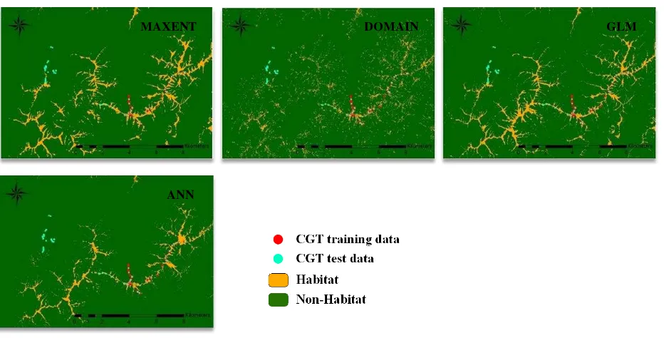
The test results of kappa values for the four modeling methods for each of three scale designs are shown in table 3. As base model in SD-1, accuracy assessment results indicated that kappa values with MAXENT (0.70) was the best among them, followed by DOMAIN (0.62) and GLM (0.59), and ANN (0.58) was the last as these models were developed only from Tong-Feng sample set and tested by another independent Tong-Feng sample set. As shown in figure 4, predictions of MAXENT and DOMAIN models generated high potential areas of CGTs and considerably reduced the area of field survey to less than 6% (1,028 ha) of the entire study area (17,136 ha), and thus they were better suited for predicting the tree’s potential habitat (also see table 4).
Next discuss how the extrapolation ability of those models (see table 3). According to the base model, we extended prediction from one area to predict another and assessed the robustness of underlying relationships. As SD-2 and SD-3, the kappa values of these models originally from 0.58–0.70 declined sharply to about 0.3, eventually near zero, with increasing spatial distance from 0.5 km to 5.0 km as the four models were tested by independent samples from Tong-feng, Yo-Shan, and Kuan-Dau sites, respectively.
Consequently, “Tong-Feng base models” built based on four algorithms failed to pass validation by Yo-Shan and Kuan-Dau test samples despite passing validation by Tong-Feng test samples. The outcome clearly indicated that the models merely based on topographic variables are most easily measured in the field and are considerably used because of their good correlation with observed species patterns in small spatial scale. Such variables usually replace a combination of different resources and direct gradients (e.g. climate, rainfall, etc) in a simple way (Guisan et al., 1999). However, the model performed poorly on spatial extrapolation from Tong-Feng to Kuan-Dau because the topographic attributes of the two watersheds are quite different from each other. Then, the models developed from topographic variables can only be applied within a limited geographical extent without significant error.
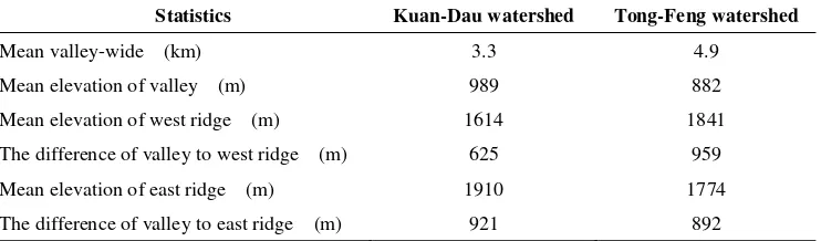
Statistics Kuan-Dau watershed Tong-Feng watershed
Mean valley-wide (km) 3.3 4.9
Mean elevation of valley (m) 989 882
Mean elevation of west ridge (m) 1614 1841
The difference of valley to west ridge (m) 625 959
Mean elevation of east ridge (m) 1910 1774
The difference of valley to east ridge (m) 921 892
Table 1. Microterrains of the two watersheds
Statistics Kuan-Dau watershed Yo-Shan Mountain Tong-Feng watershed Mean Max Min Mean Max Min Mean Max Min
Elevation (m) 1277 1640 681 1804 1884 1681 1787 2096 1157
Slope (°) 26 53 11 20 33 4 20 46 1
Aspect (°) — 359 2 — 355 60 — 359 2
Terrain Position 6 8 1 6 8 5 6 8 2
Vegetation Index 27 48 21 21 23 20 24 47 20
Hill-shade 210 254 124 167 232 124 186 253 64
Sampling Design (SD) Test Data
Kappa coefficient
MAXENT DOMAIN GLM ANN
SD-1 Tong-Feng 0.70 0.62 0.59 0.58
SD-2 Yo-Shan 0.37 0.30 0.39 0.23
SD-3 Kuan-Dau 0.00 0.03 0.00 0.00
Table 3. Comparison of the accuracies of four models for predicting CGTs potential habitats with three sets of test data
Class MAXENT DOMAN GLM ANN
Area (ha) % Area (ha) % Area (ha) % Area (ha) %
Habitat 1,051.27 6 694.47 4 719.44 4 569.54 3
Non-habitat 16,084.73 94 16,441.53 96 16,416.56 96 16,566.46 97
Sum 17,136.00 100 17,136.00 100 17,136.00 100 17,136.00 100
Table 4. The distribution statistics of three models predicting the potential habitat of CGTs
Figure 3. Perspective-viewing map showing the Huisun Forest Station
Figure 4. Sampling design 1: four models for mapping the potential habitat of CGTs in the study area
MAXENT DOMAIN GLM
5. CONCLUSIONS
To build a modeling ecological framework could tease apart complex species-environment relationship and permit more accurate description of spatial patterns and suggest directions for future research. This study represents a broad comparative exploration of species ecological characteristics with different organisms and processes respond to their environments, and the ways that these responses vary geographically.
As shown in SD-1 (small spatial scale), the performance of methods from highest to lowest was: MAXENT, DOMAIN, GLM, ANN. MAXENT and DOMAIN models were the two most capable for predicting a single species. However, the outcome clearly indicated that the models merely based on topographic variables performed poorly on spatial extrapolation from Tong-Feng to Kuan-Dau because the humidity and solar illumination affected by micro-terrain of the two watersheds are quite different from each other. Therefore, the models developed from topographic variables can only be applied within a limited geographical extent without significant error. Future studies will attempt to use variables involving spectral information associated with species extracted from high spatial, spectral resolution remotely sensed data, especially hyperspectral image data, for building a model so that it can be applied on a large spatial scale.
6. REFERNECES
Araújo, M. B. and A. Guisan, 2006. Five (or so) challenges for species distribution modelling. Biogeography, 33: 1677-1688.
Cohen, J., 1960. A coefficient of agreement for nominal scales. Educational and Psychological Measurement, 20 (1): 37-46.
Carpenter, G., A. N. Gillison and J. Winter. 1993. DOMAIN: a flexible modelling procedure for mapping potential distributions of plants and animals. Biodiversity and Conservation, 2: 667-680.
De’ath, G. and K. E. Fabricius, 2000. Classification and regression trees: a powerful yet simple technique for ecological data analysis. Ecology, 81 (11), pp. 3178-3192.
Elith, J., C. H. Graham, R. P. Anderson, M. Dudík, S. Ferrier, A. Guisan, R. J. Hijmans, F. Huettmann, J. R. Leathwick, A. Lehmann, J. Li, L. G. Lohmann, B. A. Loiselle, G. Manion, C. Moritz, M. Nakamura, Y. Nakazawa, J. Overton, M. Mcc., A. T. Peterson, S. J. Phillips, K. Richardson, R. Scachetti-Pereira, R. E. Schapire, J. Soberón, S. Williams, M. S. Wisz and N. E. Zimmermann, 2006. Novel methods improve prediction of species’ distribution from occurrence data. Ecography, 29: 129-151.
Gower, J. C., 1971. A general coefficient of similarity and some of its properties. Biometrics, 27, 857-71.
Guisan, A., S. B. Weiss and A. D. Weiss, 1999. GLM versus CCA spatial modeling of plant species distribution. Plant Ecology, 143, 107-122.
Guisan, A. and N. E. Zimmermann, 2000. Predictive habitat distribution models in ecology. Ecological Modeling, 135: 147-186.
Guisan, A., T. C. Edwards and T. Hastie, 2002. Generalized linear and generalized additive models in studies of species distributions: setting the scene. Ecological Modeling, 157: 89-100.
Hoffer, R., 1978. Biological and physical considerations in applying computer-aided analysis techniques to remote sensor data. In : Remote sensing : the quantitative approach, Swain P. H. & Davis S. M. Ed., McGraw-Hill pp 227–289.
Jensen, J. R., 2005. Introductory Digital Image Processing–A Remote Sensing Perspective, 3rd ed., Pearson Education, Inc, New Jersey.
Kumar, S. and T. J. Stohlgren, 2009. Maxent modeling for predicting suitable habitat for threatened and endangered tree Canacomyrica monticola in New Caledonia. Ecology and Natural Environment, 1(4), pp. 94-98.
Liu, Y. C., F. Y. Lu and C. H. Ou, 1994. Trees of Taiwan. Taichung, Taiwan: College of Agriculture, National Chung-Shing University, pp. 440.
Lek, S. and J. F. Guegan, 1999. Artifical neural networks as a tool in ecological modeling, an introduction. Ecological Modelling, 120, 65-73.
Lillesand, T. M., R. W. Kiefer and J. W. Chipman, 2008. Remote Sensing and Image Interpretation. 5th Edition. John Wiley & Sons. Inc., New York.
McCullagh, P. and J. A. Nelder, 1989. Generalized linear model. 2nd ed. Chapman and Hall, London, pp. 512.
Phillips S. J., R. P, Anderson and R. E. Schapire, 2006. Maximum entropy modeling of species geographic distributions. Ecological Modeling, 190: 231-259.
Phillips, S. J. and M. Dudik, 2008. Modeling of species distributions with Maxent: new extensions and a comprehensive evaluation. Ecography, 31: 161-175.
Skidmore, A. K., 1990. Terrain position as mapped from a grided digital elevation model. Geographical Information Systems. 4 (1): 33-49.