Vol. 41 (2000) 101–115
Complex dynamics in a cobweb model with adaptive
production adjustment
qTamotsu Onozaki
a,b,∗, Gernot Sieg
b,c, Masanori Yokoo
daDepartment of Economics, Asahikawa University, 3-23 Nagayama, Asahikawa, Hokkaido 079-8501, Japan bUniversity of Southern California, Los Angeles, USA
cVolkswirtschaftliches Seminar, Georg-August-Universität, Platz der Göttinger Sieben 3,
37073 Göttingen, Germany
dGraduate School of Economics, Waseda University, Nishiwaseda 1-6-1, Shinjuku, Tokyo 169-8050, Japan
Received 10 April 1998; received in revised form 19 October 1998; accepted 16 November 1998
Abstract
Chaos occurs in a nonlinear cobweb model with normal demand and supply, naive expectations and adaptive production adjustment. The model differs from existing ones in that it includes adap-tive production adjustment instead of adapadap-tive expectations. The model exhibits observable chaos (strange attractors) as well as topological chaos (horseshoes) associated with homoclinic points. As numerical simulations show, the faster suppliers adjust their production and the more inelastic demand is, the more likely the market behaves chaotically. ©2000 Elsevier Science B.V. All rights reserved.
JEL classification: D21; E32
Keywords: Nonlinear cobweb model; Adaptive production adjustment; Topological chaos; Observable chaos;
Homoclinic point
1. Introduction
A farmer decides how much to produce in a certain period before price is determined and sales revenues are received. Some economists represent anticipated sales prices by model-consistent expectations. According to their view, farmers have the true model of the
q
Financial support from the Deutsche Forschungsgemeinshaft is gratefully acknowledged. ∗Corresponding author. Tel.:+81-166-48-3121, fax:+81-166-48-8718.
E-mail addresses: [email protected] (T. Onozaki), [email protected] (G. Sieg).
product market. Many empirical researchers, for example Ito (1990) and Hey (1994), test the hypothesis that expectations are model-consistent and reject it.
Nevertheless, the farmer has to forecast the price. Experimental evidence suggests that subjects use past market prices to forecast and follow rules of thumb. Williams (1987), e.g., shows that the adaptive expectation hypothesis (including naive forecasts, which are a spe-cial case of adaptive expectations) describes expectations in an experimental double-auction market better than the extrapolative one. This result is consistent with the common behavior of the farmer who uses the most recently received price as his prediction for the next period. Such naive expectations are investigated in the formal cobweb literature starting with Kaldor (1934), Leontief (1934) and Ezekiel (1938). In models with normal supply and demand only three types of simple dynamics are possible: convergence to an equilibrium, two-period cycles or exploding oscillations. If expectations are not naive but adaptive, price behavior in the model with linear supply and demand is also simple (Nerlove, 1958). Unfortunately, the behavior of prices in agricultural markets is not so simple.1
Artstein (1983), Jensen and Urban (1984), Lichtenberg and Ujihara (1989) and Day and Hanson (1991) show that complex price behavior is possible if at least either demand or supply is non-monotonic. Hommes (1991, 1994), Finkenstädt and Kuhbier (1992) and Finkenstädt (1995) find complex behavior in normal markets with adaptive expectations when supply or demand is nonlinear.2 This literature assumes that farmers make a best (optimizing) response given current expectations.
In this paper we investigate an alternative rule which specifies that farmers adjust par-tially in the direction of the best current response. Such adjustment is a behavioral response to uncertainty and adjustment costs. In order to show that our model exhibits topological and observable chaos, we exploit some mathematical results concerning homoclinic points. The occurrence of topological chaos is proved by applying the classical Homoclinic Point Theorem which asserts that a transverse homoclinic orbit implies a horseshoe. Under dif-ferentiability, this result is a little sharper than that by the Li–Yorke Theorem in regard to continuous maps on interval. Furthermore, the occurrence of observable chaos (i.e., strange attractors) for a large set of parameter values is shown, under some minor assumption, with the aid of a recent result concerning the homoclinic bifurcation by Mora and Viana (1993). In this way, we detect chaotic behavior in a theoretically large and empirically relevant region of price elasticities of demand and adjustment speeds. The faster suppliers adjust their production and the more inelastic the demand is, the more likely the market behaves chaotically.
2. The model
At periodt, a supplier decides his productionxt+1for periodt+1. As he knows well, even a production plan that maximizes profits may turn out to be a disaster in reality. He calculates the profit maximumx˜t+1and uses it as a target of adjustment. The calculation 1Whereas many agricultural markets are regulated to stabilize prices, see for example, Finkenstädt (1995) for chaotic price movements of egg, potato and pig in Northern Germany.
is done subject to the quadratic cost function(b/2)x2, b >0 and naive price expectation, which means that his price expectation for the next period is equal to the current pricept. The resulting amount is
˜
xt+1= pt
b . (1)
He has to adjust cautiously since every theoretically advantageous change may or may not enlarge real profits. Therefore, he is assumed not to producex˜t+1immediately but to adjust adaptively his last period’s production in the direction ofx˜t+1. This is a simple hedging
rule in the uncertain real world and is expressed as the equation:
xt+1=xt +α (x˜t+1−xt) , (2)
whereα∈ (0,1)is the speed of adjustment. This equation, which can be rationalized by adjustment costs, is one of the earliest ways of incorporating adaptive processes explic-itly into economic models (Nerlove, 1958) and is often used in econometric studies of macroeconomic behaviors.3
In order to bridge the gap between a single supplier and the market as a whole, we suppose that allnsuppliers are homogeneous and behave identically. Therefore, the aggregate supply Xis given by
Xt =nxt. (3)
We assume the following monotonic inverse demand function with constant price elasticity of 1/β(β >0):
pt = c
Ytβ
, (4)
whereYt is demand at periodt andcis a positive shift parameter, which can be regarded as the extent of the market. Finally, price is set so that the market clears at each period:
Yt =Xt. (5)
Summarizing the model, we substitute Eqs. (1) and (3)–(5) into Eq. (2) and obtain the one-dimensional, discrete-time dynamical equation:
Xt+1=(1−α)Xt+ αcn
bXtβ
. (6)
To make the analysis below easier, let us consider the variable transformation:
Xt :=
As the transformation is linear, Xt behaves periodically if zt does so, andXt behaves aperiodically ifzt does so, regardless of the number of suppliersn, the slope of marginal costband the extent of the marketc. These parameters change the value ofzt into that of Xt through the scalar(b/cn)−1/(1+β). Essential parameters for the qualitative behavior of our model are the adjustment speed of productionαand price elasticity of demand 1/β. In what follows, we concentrate only on the dynamics of Eq. (7).
3. Analysis of the model
Our model (7) can be reformulated by the two-parameter family of mapsfα,β:R++→
R++as
The first and second derivatives are calculated as
f′(z)=1−α− αβ
z1+β, f
′′(z)=αβ(1+β)
z2+β >0, z∈R++,
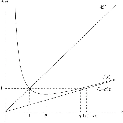
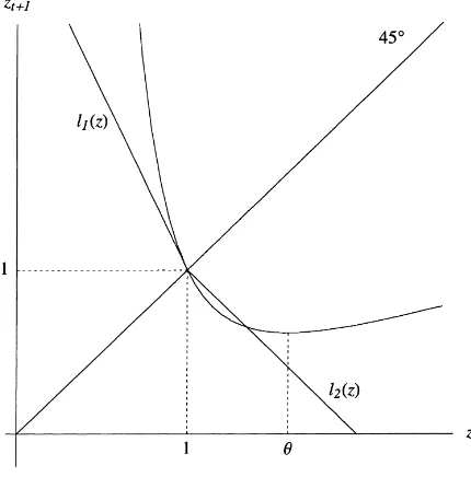
which imply thatf is a strictly convex and unimodal function onR++(see Fig. 1) with its minimum at the critical point
The fixed point is a repeller if
f′(1)=1−α−αβ <−1,
which is equivalently rewritten as
β > 2−α
α . (9)
In the following subsections we present two propositions concerning the complex behav-ior of our model. The proofs and the related fundamental notions of symbolic dynamics are given in the Appendix.
3.1. Existence of horseshoes
Fig. 1. Graph of the map (8).
existence of a horseshoe is assured by that of a transverse homoclinic point. We say that a map exhibits topological chaos either if it has a horseshoe or, alternatively, if the topological entropy of the map is positive.4 Although a map restricted on horseshoes behaves in a complicated way, the existence of horseshoes itself does not assure complex dynamics in the long run; the economic system may eventually settle down to a periodic motion even if horseshoes are present. Nevertheless, horseshoes may often generate long-lasting complicated transient dynamics, and even small external shocks are likely to give rise to erratic motions of a system which are otherwise periodic in the long run. Finding horseshoes in our model is, therefore, not insignificant even from an empirical viewpoint.
Our result is summarized as follows:
Proposition 1. Fix anα ∈ (0,1)arbitrarily. Then there exists a numberβ¯ = ¯β(α) > (2−α)/αsuch thatfβ in Eq. (8) has a horseshoe for eachβ ≥ ¯β.
One of the important features of a horseshoe (more precisely, a hyperbolic set) is the stability of the associated map againstCr-perturbations (r ≥ 1) (see e.g. de Melo and van Strien (1993), p. 225, Theorem 2.3). Roughly speaking, once the economic system described byfβ possesses horseshoes, they will be preserved despite small changes in the underlying economic structure.
3.2. Existence of strange attractors
Next we present a proposition which states that, under some generic condition, our model frequently exhibits observable chaos in the sense of strange attractors. While horseshoes do not assure complex dynamics in the long run, strange attractors do assure that we can observe erratic behavior for some large set of initial conditions. Hence, frequent occurrence of observable chaos seems to be useful in explaining irregular behavior of economic time series.
To state our proposition, we first introduce some basic notions.
Definition. A compact invariant setA ⊂ Rfor f is called an attractor if its stable set Ws(A) = {z ∈ R|limn→∞d(fn(z),A) =0}contains a nonempty interior andf has a
dense orbit inA. An attractorAhere is said to be strange if it contains a dense orbit with positive Lyapunov exponent, i.e., there is a pointz ∈ Afor which{fn(z)}
n≥0 = Aand limn→∞n−1Pni=1log|f′(fi−1(z))|>0.
Strange attractors will appear via homoclinic bifurcation, that is, when a non-degenerate homoclinic tangency unfolds generically. In other words, they will appear when the critical pointθ (β)withf′′(θ )6=0 which is contained in a homoclinic orbit to the repellerz∗=1 for someβ =β∗passes throughz∗at non-zero speed for some iterate offβ asβ varies. Formally,(d/dβ)fβn(θ (β))6=0 atβ=β∗for somenwithfβn∗(θ (β∗))=1. See Mora and Viana (1993) for a full explanation.
The following result shows that our model may exhibit observable chaos for measure-theoretically large sets of parameter values.
Proposition 2. For anyα∈(0,1),there is generically a positive measure set of parameter values ofβ, E⊂R+,such that for everyβ ∈Ethe mapfβ exhibits a strange attractor.
4. Numerical simulations of the model
In this section we perform some numerical simulations and show that those are supported by the theoretical results in the previous section.
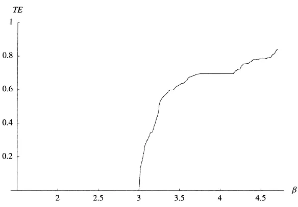
First we depict the standard, one-parameter bifurcation plot of Eq. (8) with respect to β in Fig. 2 and the corresponding topological entropy (TE) and Lyapunov exponent (LE) in Figs. 3 and 4.5 Intuitively, topological entropy measures the exponential growth rate of the number of foldings of the graph of thenth iterate of a map. By definition TE≥0, and if TE>0 then the map exhibits topological chaos. From Fig. 3 we can observe that topological chaos occurs in our model for values ofβlarger thanβTE>0≈3.0008. Propo-sition 1 states that our model may exhibit topological chaos whenβ satisfies the condi-tion (9). We can confirm this as follows: the value ofαused in the calculation of TE is 0.7 and substituting intoβ = (2−α) /α givesβˆ ≈ 1.857 < βTE>0 which is found in Fig. 2.6
5To calculate topological entropy, we utilized the algorithm presented by Block et al. (1989).
6βˆis exactly the period-doubling bifurcation value at which a single stable fixed point splits into a stable period-2
Fig. 2. Bifurcation diagram with respect toβ(1.5≤β≤4.7)withα=0.7.
Fig. 3. Graph of topological entropy corresponding to Fig. 1 withα=0.7. Topological entropy is measured using base 2 logarithms so that the vertical axis is [0,1]. A positive value for topological entropy indicates topological chaos.
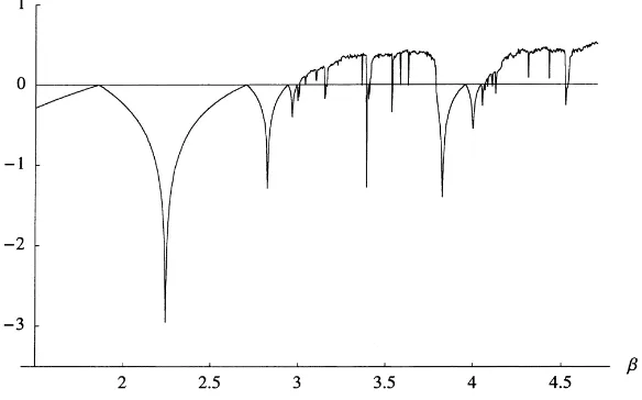
Fig. 4. Graph of Lyapunov exponent corresponding to Fig. 1 withα=0.7. A positive value of the Lyapunov exponent indicates observable chaos.
As stated in the previous section, the observable motions may be indeed periodic even if topological chaos is present. Comparing Figs. 2 and 3, it is realized that in the region of TE>0 there exist windows of periodic behavior. On the other hand, if there appear periodic motions thenLE≤0.Therefore, we can classify chaos to be present in our model as follows:
TE >0 : topological chaos (
LE >0 : observable chaos,
LE≤0 : windows (latent chaos).
In addition, the Schwarzian derivative off atzis
Sf (z)= −αβ(1+β)
αβ(β−1)+2(1−α)(2+β)z1+β 2(α−1)z2+β+αβz2 ,
and it is negative if Eq. (9) is satisfied. Therefore,f has at most one periodic attractor.7 As mentioned above, the essential parameters in our model areαandβ. Thus a question arises here: what happens to the above bifurcation plot ifαalso varies? To answer this, we draw two kinds of 2-parameter diagrams after the manner of Gallas and Nusse (1996): one is an iso-period plot and the other is an observable chaos plot. The former is the union of all iso-period-pplots forp∈[1,p¯]⊂N(in this paperp¯=64). And each iso-period-pplot is made of the set in the parameter space such that for each element in this set the trajectory through some fixed initial pointx0converges to a stable period-pcycle. The latter consists of the set in the parameter space such that for each element in this set the orbit through
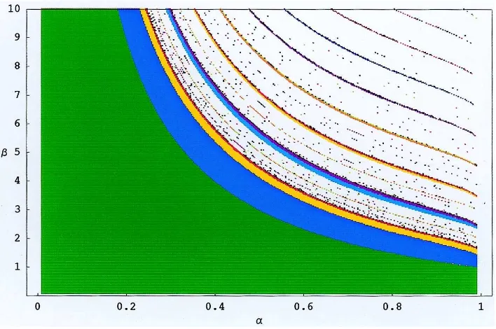
Fig. 5. Iso-period plot for the map (8). The green area corresponds to period-1 cycles (a stable fixed point), the dark blue area to period-2 cycles, the yellow area to period-4 cycles, and the red area to period-8 cycles. The blue and magenta areas correspond to period-3 and period-6 cycles.
some fixed initial pointx0is observably chaotic in the sense that it has a positive Lyapunov exponent.
We consider the regionK = {(α, β)|0< α <1,0< β≤10}. The resulting iso-period plot is shown in Fig. 5. In this figure, the green area exhibits pairs of parameter values for which every trajectory converges to a unique stable fixed point. The dark blue area consists of pairs of parameter values for which every trajectory converges to a period-2 cycle. The blue area corresponds to a period-3 cycle, the yellow area corresponds to a period-4 cycle, the magenta area corresponds to a period-6 cycle, and the red area corresponds to a period-8 cycle, etc. We emphasize that the border between the green area and the blue area is expressed by the equation β = (2−α) /α, the upper region of which satisfies Eq. (9); therefore, the fixed point of the model is unstable there.
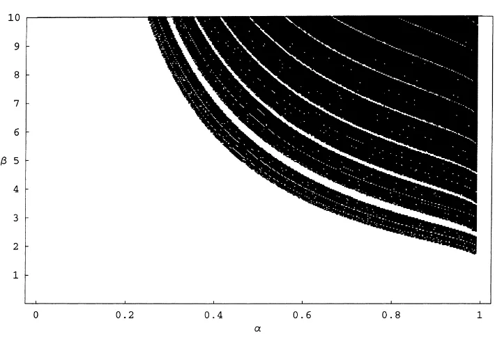
The resulting chaos plot is presented in Fig. 6. The black area in this figure is the set of parameters for which our model exhibits observable chaos in the sense of a positive Lyapunov exponent. This figure implies that observable chaos occurs whenαandβ are large. In other words, the faster suppliers adjust their production and the more inelastic demand is, the more likely the market behaves chaotically.
unfortu-Fig. 6. Observable chaos plot for the map (8). The black area is the set of(α, β)for which the model has strange attractors.
nately, as Gallas and Nusse (1996) point out, there exists no theoretical result which assures this fact.
5. Concluding remarks
We have investigated the dynamics of a nonlinear cobweb model where suppliers adjust cautiously to hedge against the uncertain world. If suppliers adapt slowly, they may stabi-lize the market. Adaptive adjustment could be a reasonable strategy to prevent large price fluctuations. Whether the cautious behavior stabilizes the market effectively depends on how much consumers change their demand as price changes.
It is well-known that price elasticities of demand for essential goods like food are relatively low. In fact, according to estimates by Pagoulatos and Sorensen (1986), the majority of US food and tobacco industries has price elasticities of less than 1/5. In such markets, chaos occurs even if adjustment is rather cautious.
Appendix
The metric space (62, d)is then compact, totally disconnected, and perfect, i.e., it is a Cantor set. The shift map σ : 62 → 62 is defined byσ ((s1, s2, . . . )) = (s2, s3, . . . ), which is referred to as the one-sided shift on two symbols.
The shift mapσ :62→62has the following properties: (i) 62contains a countably infinite set of periodic orbits; (ii) 62contains an uncountably infinite set of aperiodic orbits; (iii) the set of periodic points is dense in62;
(iv) σ : 62 → 62 is topologically mixing, i.e., for every pair of nonempty open sets U, V ⊂62, there ism≥1 such thatσn(U )∩V 6=φfor alln≥m;
(v) σ : 62 → 62is expansive, i.e., there isδ > 0 such that for anys, t ∈ 62(s 6=t ), there ism≥1 withd(σm(s), σm(t ))≥δ.
By definition, topological mixing property implies topological transitivity, and expan-siveness implies sensitive dependence on initial conditions.
LetX andY be metric spaces, and letf : X → X andg : Y → Y be continuous maps. The mapf is said to be topologically conjugate (or equivalent) togif there exists a homeomorphismh:X →Y (one-to-one, onto, continuous map with continuous inverse) such that
h◦f (x)=g◦h(x) for every x ∈X,
i.e., the diagram
top. A homoclinic orbit HOf(q, p) is said to be transverse if f′(z) 6= 0 for every z∈HOf(q, p).
Finally, we introduce an important theorem8 which is utilized to prove Proposition 1.
Theorem (Homoclinic Point Theorem forC1-Map on Interval). Letf : R → Rbe a
C1-map andp∈Rbe a repelling hyperbolic fixed point. Iff has a transverse homoclinic orbit top,then there exist a numbern∈Nand a compact set3⊂Rsuch that
(i) fn(3)=3;
(ii) p∈3;
(iii) fn|3:3→3is topologically conjugate to the one-sided full-shift on two symbols
σ :62→62,i.e., there is a homeomorphismh:3→62withh◦fn|3=σ◦h. The set3here is called a horseshoe, and if the mapf has such a set, we say that the mapf has a horseshoe. By topological conjugacy,fn|3inherits complicated dynamical properties of the shift mapσ|62described above. Furthermore, iff is a continuous map on interval and has a periodic point of period three, then for somenand some invariant set 3forfn,fn|3is topologically semi-conjugate toσ|62. See Block and Coppel (1992) for more detail.
5.1. Proof of Proposition 1
By the Homoclinic Point Theorem in the previous subsection, it suffices to show that the mapf has a transverse homoclinic orbit. To show this we have to make some preparations.
Lemma 1. The following statements hold:
(i) 0< f (θ ) <1< θ;
(ii) there is a unique pointq=q(β) > θsuch thatf (q)=1.
Proof. (i) From Eq. (9), we get the last inequality. Sincef has its global minimum atθ, we get the second inequality (see Fig. 1). (ii) Sincef (θ ) <1 andf (x) > 1 for largex,
Fig. 7. Graph of the map (8) and the piecewise linear mapLβ(z).
the strict convexity offand by the construction ofL, it is sufficient to show that forβlarge enough, the inequalityf (θ ) < l2(θ ), i.e.,
fβ(θ (β))+θ (β) <2
holds. This is verified by the fact
lim
β→∞θ (β)=βlim→∞
αβ
1−α
1/(β+1)
=1,
lim
β→∞fβ(θ (β))=βlim→∞
(1−α)θ (β)+αθ (β)−β
=1−α
which completes the proof.
Lemma 3. There is a numberβ2 > (2−α)/αsuch that for everyβ ≥ β2the following
inequality holds:
0< fβ(θ (β)) <1< θ (β) < q(β) < fβ2(θ (β)).
Proof. By Lemma 1, it suffices to show that for any arbitrarily large β, the following inequality holds:
q < f2(θ ). (A.1)
Let us define a functionlby
Again by the strict convexity off, we obtain
l◦fβ(θ (β)) < fβ2(θ (β)).
Note thatfβ(z) > (1−α)zholds for everyz∈R++(see Fig. 1), so we have
q(β) < 1 1−α.
To obtain the inequality (A.1), it is therefore sufficient to show
1
1−α ≤l◦fβ(θ (β))
for any sufficiently largeβ. Noting that
l◦fβ(θ (β))=(1−α−αβ)(1−α)θ (β)+αθ (β)−β−1+1,
we get limβ→∞l◦fβ(θ (β))= ∞. So the lemma follows.
Proof of Proposition 1. Letβ =max{β1, β2}and pickβ ≥β arbitrarily. By Lemma 3, there is a pointq′ ∈ (f (θ ),1)such that f (q′) = q. By Lemma 2, there is a sequence
{q−′i}∞i=0 ⊂ I such thatq0′ = q′, f (q−′i−1) = q−′i(i ≥ 0), and q−′i → 1(i → ∞). Hence, together withf2(q′) =1, q′ is a homoclinic point to the repeller 1. Clearly, for any homoclinic pointz ∈ HOf(q′,1) = {q′, f (q′), f2(q′) = 1} ∪ {q−′i}∞i=0, we have z6=θand sof′(z)6=0, which implies that the homoclinic orbit ofq′to 1,HOf(q′,1), is transverse. By the Homoclinic Point Theorem, the statement is proved.
5.2. Proof of Proposition 2
To find the abundance of strange attractors for the family of maps{fβ}β, we exploit the theorem by Mora and Viana (1993), Theorem C.
Proof of Proposition 2. We show that the (non-degenerate) critical pointθ (β)is contained in the homoclinic orbit of the repelling fixed pointz∗=1 for some sequence ofβ-values. Note first that the critical pointθis always non-degenerate, i.e.,f′′(θ )6=0, sincef′′(x) >0 for allx∈R++.
We can observe that there is a sequence of eventually fixed points depending smoothly onβ,
Q(β)={qi(β)|qi(β)=fβ(qi+1(β)) for i∈N, q=q1< q2<· · ·< qn<· · · }, whereqi(β)→(1−α)−i <∞asβ → ∞for everyi∈N.
fβm∗(θ (β∗))6=1 form < n. Hence, the non-degenerate critical pointθ (β∗)lies in a homo-clinic orbit to the fixed pointz∗ =1 (homoclinic tangency). Since(∂/∂β)f (x, β)=0 if and only ifx =1, we may generically assume that(d/dβ)fβn(θ (β))6=0 atβ=β∗, which implies that, in our case, this homoclinic tangency unfolds generically. By Theorem C in Mora and Viana (1993), the statement of Proposition 2 follows.
References
Artstein, Z., 1983. Irregular cobweb dynamics. Economics Letters 11, 15–17 . Block, L.S., Coppel, W.A., 1992. Dynamics in One Dimension. Springer, Berlin.
Block, L., Keesling, J., Li, S., Peterson, K., 1989. An improved algorithm for computing topological entropy. Journal of Statistical Physics 55, 929–939.
Day, R.H., 1998. Adapting, learning and economizing. In: Dopfer, K. (Ed.), Evolutionary Principles in Economics. Day, R.H., Hanson, K.A., 1991. Cobweb chaos. In: Kaul, T.K., Sengupta, J.K. (Eds.), Economic Models. Estimation
and Socioeconomic Systems, Essays in honor of Karl A. Fox, North-Holland, Amsterdam.
Devaney, R.L., 1989. An Introduction to Chaotic Dynamical Systems, 2nd ed. Addison-Wesley, Reading. Ezekiel, M., 1938. The Cobweb theorem. Quarterly Journal of Economics 52, 255–280.
Finkenstädt, B., 1995. Nonlinear Dynamics in Economics: A Theoretical and Statistical Approach to Agricultural Markets. Springer, Berlin.
Finkenstädt, B., Kuhbier, P., 1992. Chaotic dynamics in agricultural markets. Annals of Operations Research 37, 73–96.
Gallas, J.A.C., Nusse, H.E., 1996. Periodicity versus chaos in the dynamics of cobweb models. Journal of Economic Behavior and Organization 29, 447–464.
Hey, J.D., 1994. Expectations formation, rational or adaptive or . . .? Journal of Economic Behavior and Organization 25, 329–349.
Hommes, C.H., 1991. Adaptive learning and roads to chaos, The case of the cobweb. Economics Letters 36, 127–132.
Hommes, C.H., 1994. Dynamics of the cobweb model with adaptive expectations and nonlinear supply and demand. Journal of Economic Behavior and Organization 24, 315–335.
Ito, T., 1990. Foreign exchange rate expectations, Micro survey data. American Economic Review 81, 365–370. Jensen, R.V., Urban, R., 1984. Chaotic price behavior in a nonlinear cobweb model. Economics Letters 15,
235–240.
Kaldor, N., 1934. A classificatory note on the determinateness of equilibrium. Review of Economic Studies 1, 122–136.
Leontief, W.W., 1934. Verzögerte Angebotsanpassung und partielles Gleichgewicht. Zeitschrift für Nationalökonomie 5, 670–677.
Lichtenberg, A.J., Ujihara, A., 1989. Application of nonlinear mapping theory to commodity price fluctuations. Journal of Economic Dynamics and Control 13, 225–246.
Lorenz, H.-W., 1993. Nonlinear Dynamical Economics and Chaotic Motion, 2nd, revised and enlarged edition. Springer, Berlin.
de Melo, W., van Strien, S., 1993. One-Dimensional Dynamics. Springer, Berlin. Mora, L., Viana, M., 1993. Abundance of strange attractors. Acta Mathematica 171, 1–71 .
Nerlove, M., 1958. Adaptive expectations and cobweb phenomena. Quarterly Journal of Economics 72, 227–240. Pagoulatos, E., Sorensen, R., 1986. What determines the elasticity of industry demand. International Journal of
Industrial Organization 4, 237–250.