Directory UMM :Journals:Journal_of_mathematics:EJQTDE:

Electronic Journal of Qualitative Theory of Differential Equations 2005, No. 14, 1-23,http://www.math.u-szeged.hu/ejqtde/

On the unique continuation property for a nonlinear

dispersive system

Alice Kozakevicius

∗

_&

_{Octavio Vera}

†

Abstract

We solve the following problem: If (u, v) = (u(x, t), v(x, t)) is a solution of the Dispersive Coupled System with t1 < t2 which are sufficiently smooth and such that: supp u(. , tj) ⊂ (a, b) and

suppv(. , tj)⊂(a, b),− ∞< a < b <∞, j= 1,2. Then u≡0 andv≡0.

Keywords and phrases: Dispersive coupled system, evolution equations, unique continuation property.

1

Introduction

This paper is concerned with unique continuation results for some system of nonlinear evolution equation. Indeed, a partial differential equationLu= 0 in some open, connected domain Ω ofRn_{is said to have the} weak unique continuation property (UCP) if every solution uof _Lu= 0 (in a suitable function space), which vanishes on some nonempty open subset of Ω vanishes in Ω. We study the UCP of the system of nonlinear evolution equations

(1.1)

∂tu+∂x3u+∂x(u v2) = 0 (P1)

∂tv+∂x3v+∂x(u2v) +∂xv= 0 (P2)

with 0_≤x_≤1, t_≥0 and whereu=u(x, t), v=v(x, t) are real-valued functions of the variablesxand

t.The general system is

(1.2)

∂tu+∂x3u+∂x(upvp+1) = 0

∂tv+∂x3v+∂x(up+1vp) = 0

with domain −∞< x < ∞, t≥ 0 and whereu= u(x, t), v =v(x, t) are real-valued functions of the variablesxandt.The powerpis an integer greater than or equal to one. This system appears as a special case of a broad class of nonlinear evolution equations studied by Ablowitzet al. [1] which can be solved by the inverse scattering method. It has the structure of a pair of Korteweg - de Vries(KdV) equations coupled through both dispersive and nonlinear effects. A system of the form (1.2) is of interest because it models the physical problem of describing the strong interaction of two-dimensional long internal gravity waves propagating on neighboring pynoclines in a stratified fluid, as in the derived model by Gear and Grimshaw [8]. Indeed,

(1.3)



  

  

∂tu+∂x3u+a3∂x3v+u ∂xu+a1v ∂xv+a2∂x(u v) = 0 in x∈R, t≥0

b1∂tv+∂x3v+b2a3∂3xu+v ∂xv+b2a2u ∂xu+b2a1∂x(u v) = 0

u(x,0) =ϕ(x)

v(x,0) =ψ(x)

whereu=u(x, t), v=v(x, t) are real-valued functions of the variablesxandtanda1, a2, a3, b1, b2are real constants withb1 >0 and b2 >0. Mathematical results on (1.3) were given by J. Bonaet al. [4].

∗_{Departamento de Matem´atica, CCNE, Universidade Federal de Santa Maria, Faixa de Camobi, Km 9, Santa Maria, RS,}

Brasil, CEP 97105-900. E-mail: alicek@smail.ufsm.br: This research was partially supported by CONICYT-Chile through the FONDAP Program in Applied Mathematics (Project No. 15000001).

†_{Departamento de Matem´atica, Universidad del B´ıo-B´ıo, Collao 1202, Casilla 5-C, Concepci´on, Chile. E-mail:}

They proved that the coupled system is globally well posed inHm_(R)

×Hm_{(R),for anym}

≥1 provided |a3|<1/√b2.Recently, this result was improved by F. Linares and M. Panthee [19].Indeed, they proved the following:

Theorem 1.1. For any (ϕ, ψ) _∈ Hm_(R)

×Hm_{(R), with m}

≥ −3/4 and any b _∈ (1/2,1), there ex-istT =T(_||ϕ_||Hm,||ψ||_Hm)and a unique solution of(1.3)in the time interval [−T, T]satisfying

u, v_∈C([₋T, T];Hm_(R)),

u, v∈Xm, b⊂Lpx Loc(R;L2t(R)) for 1≤p≤ ∞,

(u2₎

x,(v2)x∈Xm, b−1,

ut, vt∈Xm−3, b−1

Moreover, given t _∈ (0, T), the map (ϕ, ψ) _7→ (u(t), v(t)) is smooth from Hm_(R)

×Hm_{(R) to}

C([₋T, T];Hm_(R))

×C([₋T, T];Hm_(R)).

Similar results in weighted Sobolev spaces were given by [29,30] and references therein. In 1999, Alarc´ on-Angulo-Montenegro [2] showed that the system (1.2) is global well-posedness in the classical Sobolev spaceHm_(R)

×Hm_{(R), m}

≥1.For the UCP the first results are due to Saut and Scheurer [24].They con-sidered some dispersive operators in one space dimension of the typeL=i Dt+α i2k+1D2k+1+R(x, t, D)

where α ₆= 0, D = 1_{i ∂x}∂ , Dt = 1_{i ∂t}∂ and R(x, t, D) = P_j2k₌₀rj(x, t)Dj, rj ∈L∞loc(R;L2loc(R)). They

proved that if u_∈ L2

loc(R;H

2k+1

loc (R)) is a solution of Lu = 0, which vanishes in some open set Ω1 of R_x×R_{t,thenuvanishes in the horizontal component of Ω1. As a consequence of the uniqueness of the} solutions of the KdV equation inL∞

loc(R;H3(R)),their result immediately yields the following:

Theorem 1.2. If u_∈L∞

loc(R;H3(R))is a solution of the KdV equation

ut+uxxx+u ux= 0 (1.4)

and vanishes on an open set ofR_x×R_{t,then u(x, t) = 0for x∈}R_{, t∈}R_.

In 1992, B. Zhang [32] proved using inverse scattering transform and some results from Hardy func-tion theory that if u ∈ L∞Loc(R;Hm(R)), m > 3/2 is a solution of the KdV equation (1.4), then it

cannot have compact support at two different moments unless it vanishes identically. As a consequence of the Miura transformation, the above results for the KdV equation (1.4) are also true for the modified Korteweg-de Vries equation

ut+uxxx−u2ux= 0. (1.5)

A variety of techniques such as spherical harmonics [26],singular integral operators [20],inverse scattering [31],and others have been used. However the Carleman methods which consists in establishing a priori estimates containing a weight has influenced a lot the development on the subject.

This paper is organized as follows: In section 2, we prove two conserved integral quantities and local existence theorem. In section 3, we prove the Carleman estimate and Unique Continuation Property. In section 4, we prove the main theorem.

2

Preliminaries

We consider the following dispersive coupled system

(P)



    

    

∂tu+∂x3u+∂x(u v2) = 0 (P1)

∂tv+∂x3v+∂x(u2v) +∂xv= 0 (P2)

u(x,0) =u0(x) ; v(x,0) =v0(x) (P3)

∂k

xu(0, t) =∂xku(1, t), k= 0,1,2. (P4)

∂k

with 0_≤x_≤1, t_≥0 and whereu=u(x, t), v=v(x, t) are real-valued functions of the variablesxandt.

Notation. We write time derivative byut=∂u_∂t =∂tu.Spatial derivatives are denoted byux= ∂u_∂x =∂xu,

uxx= ∂

2

u ∂x2 =∂

2

xu, uxxx= ∂

3

u ∂x3 =∂

3

xu.

If E _{is any Banach space, its norm is written as || · ||E. For 1 ≤ p ≤ +∞, the usual class of p}th -power Lebesgue-integrable (essentially bounded if p = +∞) real-valued functions defined on the open set Ω inRn_{is written byL}p_{(Ω) and its norm is abbreviated as|| · ||p.The Sobolev space ofL}2_-functions whose derivatives up to order m also lie in L2 _{is denoted by H}m_{. We denote [H}m1_{(Ω), H}m2_{(Ω)] =}

H(1−θ)m1+θm2_{(Ω) for all m}

i > 0(i = 1,2), m2 < m1, 0 < θ < 1 (with equivalent norms) the in-terpolation of Hm_{(Ω)-spaces. If a function belongs, locally, to L}p _{or H}m _{we write f ∈ L}p

loc or

f ∈Hlocm. C(0, T;E) denote the class of all continuous mapsu: [0, T]→ E equipped with the norm

||u_||C(0, T;E) = sup0≤t≤T||u||E. u(x, t) ∈C3,1(R2) if ∂xu, ∂x2u, ∂x3u, ∂tu∈ C(R2). u(x, t)∈ C03,1(R2) if

u_∈C3,1_(R2_{) and u with compact support.}

Throughout this papercis a generic constant, not necessarily the same at each occasion(will change from line to line), which depends in an increasing way on the indicated quantities. The next proposition is well known and it will be used frequently

Proposition 2.1. Let K be a non empty compact set and F a close subset of R _{such thatK∩F =∅.}

Then there isψ∈C0∞(R)such that ψ= 1 inK, ψ= 0in F and0≤ψ(x)≤1, ∀x∈R.

Definition 2.2. Let L be an evolution operator acting on functions defined on some connected open setΩof R2₌R_x×R_{t. Lis said to have the horizontal unique continuation property if every solutionu}

ofLu= 0 that vanishes on some nonempty open setΩ1⊂Ω vanishes in the horizontal component of Ω1

inΩ, i. e., inΩh={(x, t)∈Ω/∃x1, (x1, t)∈Ω1}.

Lemma 2.3. The equation(P)has the following conserved integral quantities, i. e.,

d dt

Z 1

0

(u2+v2)dx= 0, (2.1)

d dt

Z 1

0

u2v2−(u2x+vx2) +v2

dx= 0. (2.2)

Proof. (2.1) Straightforward. We show (2.2). Multiplying (P1) by (u v2+uxx) and integrating over

x_∈(0,1) we have

1 2

Z 1

0 (u2₎

tv2dx+

Z 1

0

uxxutdx+

Z 1

0

(u v2_)u

xxxdx

+1 2

Z 1

0 (u2

xx)xdx+

1 2

Z 1

0

[(u v2₎2_]

xdx+

Z 1

0 (u v2₎

xuxxdx= 0.

Each term is treated separately integrating by parts

1 2

Z 1

0

(u2)tv2dx−

Z 1

0

uxuxtdx−

Z 1

0

(u v2)xuxxdx

+1 2

Z 1

0

(u2xx)xdx+1

2

Z 1

0

[(u v2)2]xdx+

Z 1

0

(u v2)xuxxdx= 0

where

1 2

Z 1

0

(u2)tv2dx−

1 2

Z 1

0

Similarly, multiplying (P2) by (u2v+vxx+v) and integrating overx∈(0,1) we have

Each term is treated separately, integrating by parts

1

adding (2.3) and (2.4), we have

1

Proof. Forǫ >0,we approximate the system (P) by the parabolic system

We rewrite the above equations in a more friendly way as

Adding (2.11) and (2.12) we obtain

1

Where in particular

hence

On the other hand, using the Lemma 2.4 and performing appropriate calculations we obtain

We also have

We calculate in similar form the terms

This way we have

Hence from (2.14)-(2.15) and (2.19)-(2.20) we have the existence of subsequencesuǫj

def

= uǫandvǫj

def

= vǫ

such that

uǫ⇀ u∗ weakly in L∞(0, T;L2(0,1))֒→L2(0, T;L2(0,1)) =L2(Q)

vǫ⇀ v∗ weakly in L∞(0, T;L2(0,1))֒→L2(0, T;L2(0,1)) =L2(Q)

∂uǫ

∂x

∗

⇀ ∂u

∂x weakly in L

∞_{(0, T;L}2_(0,1))֒

→L2(0, T;L2(0,1)) =L2(Q)

∂vǫ

∂x

∗

⇀ ∂v

∂x weakly in L

∞_{(0, T;L}2_(0,1))֒

→L2_{(0, T;L}2_{(0,1)) =L}2_(Q)

from the equation (R) we deduce that

∂uǫ

∂t

∗

⇀ ∂u

∂t weakly in L

2_{(0, T;H}−2_(0,1))

∂vǫ

∂t

∗

⇀ ∂v

∂t weakly in L

2_{(0, T;H}−2_(0,1)).

By other hand, we haveH1_(0,1)֒→c _L2_(0,1)֒→H−2_{(0,1).Using Lions-Aubin’s compactness Theorem}

uǫ→u strongly in L2(Q)

vǫ→v strongly in L2(Q).

Then

∂x(uǫv2ǫ) = 2uǫvǫ∂vǫ

∂x + ∂uǫ

∂x vǫvǫ−→2u v ∂v ∂x+

∂u

∂xv v=∂x(u v

2_{) in}

D′_(0,1).

The other terms are calculated in a similar way and therefore we can pass to the limit in the equation (R).Finally, u, v are solutions of the equation (P) and the theorem follows.

3

Carleman’s estimate and unique continuation

property

We consider the equation (P), then

(Q)

∂tu+∂x3u+v2ux+ 2u v vx= 0

∂tv+∂x3v+ 2u v ux+u2vx+vx= 0

We rewrite the above equations as

∂t

u v

+∂x3

u v

+

v2 _{2u v} 2u v u2

∂x

u v

+

0 0 0 1

∂x

u v

=

0 0

LetU=U(x, t),

U =

u v

; B(U) =

v2 _{2u v} 2u v u2

=

f1 f2

f3 f4

; C=

0 0 0 1

Hence in (Q) we obtain

Ut+Uxxx+ (B(U) +C)Ux= 0, 0≤x≤1, t≥0 (3.1)

Then

LU =

I∂t+I ∂x3+B(U)∂x

U. (3.3)

System (3.1) may be written as

LU = 0 (3.4)

with

L=I∂t+I ∂x3+B(U)∂x. (3.5)

We see in (3.1) and (3.4) that the system (3.1) may be written as_LU = 0 where the operator_Lis given in (3.5). It has the form:

L=

L1 f2∂x

f3∂x L2

(α)

with

L1 = ∂t+∂x3+f1∂x (3.6)

L2 = ∂t+∂x3+f4∂x. (3.7)

Proposition 3.1 (Carleman’s Estimate). Let δ > 0, B_{δ = {(x, t) ∈} R2_{/ x}2_+t2 _{< δ}2_{}, ϕ(x, t) =} (x−δ)2_+δ2_t2_{and the differential operatorLdefined by (3.5). Assume thatf}

k ∈L∞(Bδ), k= 1,2,3,4.

Then

3τ2

Z

Bδ|

Φx|2e2τ ϕdx dt+ 12τ3

Z

Bδ|

Φ_|2e2τ ϕdx dt_≤2

Z

Bδ|L

Φ_|2e2τ ϕdx dt (3.8)

for any Φ∈C0∞(Bδ)×C0∞(Bδ)andτ >0 large enough.

Proof. We consider the operatorP1=∂t+∂x3, then using the Treve inequality

96τ2

Z

Bδ|

Φx|2e2τ ϕdx dt ≤

Z

Bδ|

P1Φ|2e2τ ϕdx dt (3.9)

384τ3Z

Bδ|

Φ_|2_e2τ ϕ_{dx dt}

≤

Z

Bδ|

P1Φ|2e2τ ϕdx dt (3.10)

whenever Φ_∈C∞

0 (Bδ) andτ >0.Adding up the inequalities (3.9) and (3.10), we obtain

96τ2

Z

Bδ|

Φx|2e2τ ϕdx dt+ 384τ3

Z

Bδ|

Φ_|2e2τ ϕdx dt_≤2

Z

Bδ|

P1Φ|2e2τ ϕdx dt

for any Φ_∈C∞

0 (Bδ) andτ >0. Then

12τ2

Z

Bδ|

Φx|2e2τ ϕdx dt+ 48τ3

Z

Bδ|

Φ_|2e2τ ϕdx dt_≤ 1

4

Z

Bδ|

P1Φ|2e2τ ϕdx dt (3.11)

for any Φ∈C0∞(Bδ) andτ >0. Similarly, we have for the operatorP1=∂t+∂x3.

12τ2

Z

Bδ|

Ψx|2e2τ ϕdx dt+ 48τ3

Z

Bδ|

Ψ_|2e2τ ϕdx dt_≤1

4

Z

Bδ|

P1Ψ|2e2τ ϕdx dt (3.12)

for any Ψ∈C0∞(Bδ) and τ >0.On the other hand,

Z

Bδ|

f1Φx|2e2τ ϕdx dt≤ ||f1||2L∞₍

Bδ)

Z

Bδ|

Letτ_≥ √6

12 ||f1||L∞₍

Bδ),thenτ2≥₂₄1 ||f1||L2∞₍

Bδ).This way in (3.9) we have

Z

Bδ|

P1Φ|2e2τ ϕdx dt ≥ 96τ2

Z

Bδ|

Φx|2e2τ ϕdx dt≥96

1 24||f1||

2

L∞₍

Bδ)

Z

Bδ|

Φx|2e2τ ϕdx dt

= 4_||f1||2L∞ (Bδ)

Z

Bδ|

Φx|2e2τ ϕdx dt≥4

Z

Bδ|

f1Φx|2e2τ ϕdx dt (using (3.13))

hence

Z

Bδ|

f1Φx|2e2τ ϕdx dt≤

1 4

Z

Bδ|

P1Φ|2e2τ ϕdx dt. (3.14)

Then adding (3.12) and (3.14) we have

Z

Bδ|

f1Φx|2e2τ ϕdx dt+ 12τ2

Z

Bδ|

Φx|2e2τ ϕdx dt+ 48τ3

Z

Bδ|

Φ_|2_e2τ ϕ_{dx dt}

≤ 1₂

Z

Bδ|

P1Φ|2e2τ ϕdx dt. (3.15)

But L1 = ∂t+∂x3+f1∂x = P1+f1∂x. Then P1Φ = L1Φ−f1Φx and |P1Φ|2 ≤2|L1Φ|2+ 2|f1Φx|2.

Hence, in (3.15)

Z

Bδ|

f1Φx|2e2τ ϕdx dt+ 12τ2

Z

Bδ|

Φx|2e2τ ϕdx dt+ 48τ3

Z

Bδ|

Φ|2_e2τ ϕ_{dx dt}

≤

Z

Bδ|

L1Φ|2e2τ ϕdx dt+

Z

Bδ|

f1Φx|2e2τ ϕdx dt

then

12τ2Z

Bδ|

Φx|2e2τ ϕdx dt+ 48τ3

Z

Bδ|

Φ_|2_e2τ ϕ_{dx dt}

≤

Z

Bδ|

L1Φ|2e2τ ϕdx dt. (3.16)

for any Φ_∈C∞

0 (Bδ) andτ ≥

√

6

12 ||f1||L∞₍

Bδ).Performing similar calculations with (3.12) and the operator

L2,we obtain

12τ2

Z

Bδ|

Ψx|2e2τ ϕdx dt+ 48τ3

Z

Bδ|

Ψ|2_e2τ ϕ_{dx dt}

≤

Z

Bδ|

L2Ψ|2e2τ ϕdx dt. (3.17)

for any Ψ_∈C∞

0 (Bδ) andτ ≥

√

6

12 ||f4||L∞₍

Bδ).Summing up (3.16) and (3.17), we have

3τ2

Z

Bδ|

Θx|2e2τ ϕdx dt+ 12τ3

Z

Bδ|

Θ|2_e2τ ϕ_{dx dt}

≤1₄

Z

Bδ

(|L1Φ|2+|L2Ψ|2)e2τ ϕdx dt. (3.18)

Whenever

Θ =

Φ Ψ

∈C0∞(Bδ)×C0∞(Bδ) and τ≥Max

(√

6

12 ||f1||L∞(Bδ); √

6

12 ||f4||L∞(Bδ)

)

.

Similarly, sincef2, f3∈L∞(Bδ) and according to Land (3.6), (3.7) we have

|LΘ_|2₌

|L1Φ +f2Ψx|2+|L2Ψ +f3Φx|2

Then we can addf2Ψx toL1Φ andf3Φx to L2Ψ in (3.18), and obtain Carleman’s estimate (3.8) when

Θ =

Φ Ψ

andτ satisfyingτ≥Maxn√₁₂6||f1||L∞ (Bδ);

√

6

12 ||f4||L∞ (Bδ),

√

6

6 ||f2||L∞ (Bδ);

√

6

6 ||f3||L∞ (Bδ)

o

.

Remark 3.2. The estimate (3.8) is invariant under changes of signs of any term inL1 orL2.

Corollary 3.3. Assume that, in addition to the hypotheses of Proposition 3.1, we have for any T >0

anda >0 that

V =

ξ η

∈L2(₋T, T; H3(₋a, a)_×H3(₋a, a)).

Vt=

ξt

ηt

∈L2(₋T, T; H3(₋a, a)_×L2(₋a, a)).

and that suppξ and suppη are compact sets in B_{δ. Then, the estimate (3.8) holds with V instead of}

Θ =

Φ Ψ

Indeed,

3τ2

Z

Bδ|

Vx|2e2τ ϕdx dt+ 12τ3

Z

Bδ|

V|2_e2τ ϕ_{dx dt}

≤2

Z

Bδ|L

V|2_e2τ ϕ_{dx dt (3.19)}

for τ >0 sufficiently large.

Proof. Choose a regularization sequence{ρǫ(x, t)}ǫ>0. Consider the functions

Vǫ=ρǫ∗V =

ρǫ∗ξ

ρǫ∗η

(∗denote the usual convolution)

Hence, the inequality (3.8) is valid replacing

Θ =

Φ Ψ

by Vǫ=

ρǫ∗ξ

ρǫ∗η

if ǫ >0 is sufficiently small.

Taking the limit asǫ→0+the result follows.

Theorem 3.4. Let T > 0, a > 0 and R = (₋a, a)_×(₋T, T). Let _L be the operator defined in (α)

and let

U =

u v

∈L2₍

−T, T; H3₍

−a, a)_×H3₍ −a, a))

be a solution of the differential equation (3.4), _LU = 0. Assume that fk ∈ L∞(R), k = 1,2,3,4 and

U _≡0whenx < t2_{in a neighborhood of(0,0).Then, there exists a neighborhood of(0,0)for whichU} ≡0.

Proof. We choose a positive number δ < 1 such that B_{δ lies in the neighborhood where U ≡ 0} whenx < t2_{.Let χ∈C}∞

0 (Bδ), χ≡1 on a neighborhood N of (0,0) and set

V =χU=

χ u χ v

.

The functionV satisfies the conditions of Corollary 3.3, and_L = 0 on_N because V =U on_N. Hence by (3.19)

6τ3

Z

Bδ|

V|2_e2τ ϕ_{dx dt}

≤

Z

Bδ−N|L

V|2_e2τ ϕ_{dx dt (3.20)}

whenτ >0 is sufficiently large. On the other hand, if (x, t)∈suppV one has 0≤t2≤x < δ <1 and

ϕ(x, t) = (x−δ)2+δ2t2= (δ−x)2+δ2t2= (t2−δ)2+δ2t2

= t4₋2t2δ+δ2+δ2t2= t2[ (t2₋2δ+δ2) +δ2]

< δ2_{[ (δ}2

and whereϕ(0,0) =δ2_{.Therefore, if (x, t)}

∈supp_LV there is anǫ >0 such that ϕ(x, t)_≤δ2

−ǫ.We can choose a neighborhood_N′ _{of (0,0) at whichϕ(x, t)> δ}2

−ǫand obtain from (3.20)

Z

N′|

V_|2e2τ ϕdx dt_≤ 1

6τ3

Z

IBδ−N

|LV_|2e2τ ϕdx dt (3.21)

Taking limit in (3.21) asτ_→+_∞one deduces thatU =V _≡0 on_N′_.

Definition 3.5. By a Holmgren’s transformation we mean a transformation which is defined by ξ =

t, η=x+t2 _{and which maps the half-space x≥0 into the domain Ω ={(η, ξ)∈R}2_{: η−ξ}2_≥0}.

Corollary 3.6. Under the assumptions of Theorem 3.4, consider the curve x = µ0(t), µ0(0) = 0,

µ0 a continuously differentiable function in a neighborhood of (0,0). Suppose thatU ≡0 in the region

x < µ0(t)in a neighborhood of (0,0).Then, there exists a neighborhood of (0,0)whereU ≡0.

Proof. We consider the Holmgren transformation

(x, t)_−→(η, ξ) , η=x₋µ0(t) +t2 , ξ=t.

With this variables the functionU =U(η, ξ) satisfiesU _≡0 whenη < ξ2 _{in a neighborhood of (0,0) and} FU = 0,where

F=

∂ξ+∂η3+F1∂η f2∂η

f2∂η ∂ξ+∂η3+F4∂η

where

F1(η, ξ) =f1(x, t) + (2ξ−µ′0(ξ)) and F4(η, ξ) =f4(x, t) + (2ξ−µ′0(ξ))

Thus by using Theorem 3.4, and Holmgren’s transformation we conclude that there exists a neighborhood of (0,0) in the x t₋plane whereU _≡0.

Theorem 3.7. Let T >0andΩ = (0,1)_×(0, T).Assume that fk ∈L∞Loc(Ω), k= 1,2,3,4.Let

U =

u v

∈L2(0, T;H3(0,1)_×H3(0,1))

be a solution of the equation (3.1). If U _≡0 in an open subset Ω1 of Ω, then U ≡0 in the horizontal

componentΩh of Ω1 inΩ.

Proof. We prove the theorem for the equation (3.1) or the equivalent equation _LU = 0, where _L is the operator defined in (2.4). The proof follows as in [21] applying Corollary 3.6 and considering Remark 3.2.

Corollary 3.8. LetT >0,Ω = (0,1)×(0, T)and let

U =

u v

∈C(0, T;Hp3(0,1)×Hp3(0,1))

be a solution of equation (3.1). Suppose thatU vanishes in an open subsetΩ1 ofΩ.Then U ≡0 inΩ.

4

The Main Theorem

Lemma 4.1. Let (u, v) = (u(x, t), v(x, t)) be a solution of the coupled system equations (P) such that

sup

t∈[0,1] ||

u(. , t)_||H1_(R)<+∞ ; sup

t∈[0,1] ||

v(. , t)_||H1_(R)<+∞

and eβx_u

0∈L2(R); eβxv0∈L2(R), ∀β >0.Then eβxu∈C([0,1];L2(R)); eβxv∈C([0,1];L2(R)).

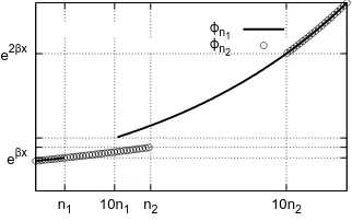
Proof. Letϕn∈C∞(R) be defined by

ϕn(x) =

(

eβ x _{, for x}

≤n e2β x _{, for x >10n}

with

ϕn(x)≤e2β x ; 0≤ϕ′n(x)≤β ϕn(x) ; |ϕ(nj)(x)| ≤βjϕn(x) j= 2,3. (4.1)

Examples.

0.95 1.2 1.45

n=0

ϕ0

eβx e2βx

0 n 10n

ϕ2

eβx e2βx

0 n 10n

ϕ3

eβx e2βx

0 n 10n

ϕ4

Figure 1: These are sample figures for different values ofn.

eβx

n1 10n1

ϕn1

e2βx

n2 10n2

ϕn2

Let

ut+uxxx+uxv2+u(v2)x= 0. (4.2)

Multiplying the equation (4.2) by u ϕn, and integrating by parts we get

Z

Integrating by parts we obtain

1

Similarly, multiplying the equation

vt+vxxx+ (u2)xv+vxu2= 0 (4.4)

by v ϕn and integrating by parts, we obtain

d

Hence, from (4.3) and (4.5)

then

d dt

Z

R

[u2+v2]ϕndx+ 3

Z

R

[u2x+vx2]ϕ′ndx−

Z

R

[u2+v2]ϕ′′′n dx

−3

Z

R

u2v2ϕ′ndx= 0

hence,

d dt

Z

R

[u2+v2]ϕndx+ 3

Z

R

[u2x+vx2]ϕ′ndx=

Z

R

[u2+v2]ϕ′ndx+ 3

Z

R

u u v v ϕ′ndx

≤β3

Z

R

[u2+v2]ϕndx+ 3β

Z

R

u u v v ϕndx. (using (4.1))

Using thatϕn ≥0 and the Holder inequality

d dt

Z

R

[u2+v2]ϕndx ≤ β3

Z

R

[u2+v2]ϕndx+ 3β||u||L∞_(R)||v||_L∞_(R)

Z

R

u v ϕndx

≤ β3

Z

R

[u2+v2]ϕndx

+ 3β_||u_||L∞₍

R)||v||L∞₍ IR)

Z

R

u2ϕndx

1/2Z

R

v2ϕndx

1/2

≤ β3

Z

R

[u2+v2]ϕndx+

3

2β||u||L∞(R)||v||L∞(IR)

Z

R

[u2+v2]ϕndx

≤

β3+3

2β||u||L∞(R)||v||L∞(R)

Z

R

[u2+v2]ϕndx

then

d dt

Z

R

[u2+v2]ϕndx≤c1

Z

R

[u2+v2]ϕndx

where c1=β3+3₂β||u||L∞₍

R)||v||L∞₍

R).Thus,

d dt

R

R[u

2_+v2_]ϕ

ndx

R

R[u2+v2]ϕndx

≤c1.

Integrating overt_∈[0,1] we have

Z t

0

d dt

R

R[u

2_+v2_]ϕ

ndx

R

R[u2+v2]ϕndx

ds≤c1t

then

Ln

R

R[u

2_+v2_]ϕ

ndx

R

R[u

2

0+v20]ϕndx

≤c1t

hence

Z

R

[u2_+v2_]ϕ

ndx≤

Z

R

[u2

0+v20]ϕndx

ec1t

thus

sup

t∈[0,1]

Z

R

[u2+v2]ϕndx≤

Z

R

[u20+v02]ϕndx

ec1

≤

Z

R

[u20+v02]e2β xdx

Now, taking n_→+_∞ we obtain

sup

t∈[0,1]

Z

R

[u2_+v2_]e2β x_dx

≤

Z

R

[u2

0+v02]e2β xdx

ec1

This way if

sup

t∈[0,1] ||

u(. , t)_||H1_(R)<∞ ; sup

t∈[0,1] ||

v(. , t)_||H1_(R)<+∞

and

eβ xu0∈L2(R) ; eβ xv0∈L2(R), ∀β >0 then

eβ x_u

∈C([0,1];L2_{(R)) ; e}β x_v

∈C([0,1];L2_(R))

with

c1=β3+ 3

2β||u||L∞(R×[0,1])||v||L∞(R×[0,1]). We have the following extension to higher derivatives.

Lemma 4.2. Let j ∈ N_{. Let (u, v) = (u(x, t), v(x, t)) be a solution of the coupled system equations} (P)such that

sup

t∈[0,1] ||

u(. , t)||Hj+1_(R)<+∞ ; sup

t∈[0,1] ||

v(. , t)||Hj+1_(R)<+∞

and

eβ x_u

0, . . . , eβ x∂xju0∈L2(R) ; eβ xv0, . . . , eβ x∂xjv0∈L2(R), ∀β >0

then

sup

t∈[0,1] ||

u(t)_||Cj−1_(R)≤c_j =c_j(u₀, c₁) ; sup

t∈[0,1] ||

v(t)_||Cj−1_(R)≤c_j=c_j(v₀, c₁)

withc1=β3+3₂β||u||L∞₍

R×[0,1])||v||L∞₍

R×[0,1]).

Lemma 4.3. If (u, v)_∈C03,1(R2)×C 3,1

0 (R2),then

||eλ xu||L8_(R2₎≤ ||eλ x{∂_t+∂_x3}u||_L8/7_(R2₎ ; ||eλ xv||_L8_(R2₎≤ ||eλ x{∂_t+∂_x3}v||_L8/7_(R2₎ for all λ∈R_{, with c independent of λ.}

Proof. Similar to those in [15].

Lemma 4.4. If (u, v)_∈C3,1_(R2₎

×C3,1_(R2_{),such that}

suppu _⊆[₋M, M]_×[0,1] ; suppv _⊆[₋M, M]_×[0,1] (4.6)

and

u(x,0) =u(x,1) = 0 and v(x,0) =v(x,1) = 0, ∀x∈R_{, (4.7)}

then

||eλ xu_||L8_(R×[0,1]) ≤ c||eλ x{∂_t+∂_x3}u||_L8/7_(R×[0,1]) (4.8)

||eλ x_v

for allλ_∈R_{, with cindependent of λ.}

Proof. Letϕǫ∈C0∞(R) with

suppϕǫ⊆[0,1]

ϕǫ(t) = 1 for t∈(ǫ,1−ǫ),

0_≤ϕǫ(t)≤1 and |ϕ′ǫ(t)| ≤c/ǫ, c constant positive.

Example.

0 1

ε 1-ε

ϕε

Let uǫ(x, t) =ϕǫ(t)u(x, t), hence

suppuǫ(x, t) ⊆ suppϕǫ(t)∩suppu(x, t)⊆suppu(x, t)⊆[−M, M]×[0,1].

Then, on one hand we have that

||eλ xuǫ||L8_(R2₎−→ ||eλ xu||_L8_(R×[0,1]) as ǫ↓0 (4.10)

and on the other hand,

{∂t+∂x3}uǫ(x, t) ={∂t+∂x3}[ϕǫ(t)u(x, t) ] =ϕǫ(t){∂t+∂x3}u+ϕ′ǫ(t)u. (4.11)

Hence,

||ϕǫ(t){∂t+∂x3}u||L8/7_(R2₎−→ ||{∂_t+∂_x3}u||_L8/7_(R2₎

and

||ϕ′ǫ(t)u||L8/7_(R2₎ = Z

IR

Z

R|

ϕ′ǫ(t)u(x, t)|8/7dx dt

7/8

=

" Z 1

0

Z M −M|

ϕ′ǫ(t)|8/7|u(x, t)|8/7dx dt

#7/8

(using (4.6))

=

" Z ǫ

0

Z M −M|

ϕ′ǫ(t)|8/7|u(x, t)|8/7dx dt+

Z 1

1−ǫ

Z M −M|

ϕ′ǫ(t)|8/7|u(x, t)|8/7dx dt

#7/8

≤ c_ǫ

" Z ǫ

0

Z M −M|

u(x, t)|8/7_{dx dt+}Z 1

1−ǫ

Z M −M|

u(x, t)|8/7_{dx dt}

#7/8

. (4.12)

Defining

G(t) =

Z M −M|

then, by (4.7) we have that G(0) =G(1) = 0. Gis continuous and differentiable with

G′(t) =8 7

Z M −M|

u(x, t)|1/7_∂

tu(x, t) sgn(u(x, t))dx

hence, G′(t) is continuous,

|G′(t)| ≤c|t| , |G′(t)| ≤c|1−t|

and

Z ǫ

0

G(t)dt+

Z 1

1−ǫ

G(t)dt_≤c ǫ2. (4.13)

Inserting (4.13) in (4.12) we have

||ϕ′ǫ(t)u||L8/7_(R2₎≤c

1

ǫǫ

7/4

→0 as ǫ_↓0

and (4.8) follows. Similarly, we obtain (4.9).

Lemma 4.5. Let (u, v)_∈C3,1_(R

×[0,1])_×C3,1_(R

×[0,1]). Suppose that

X

j≤2 |∂j

xu(x, t)| ≤Cβe−β|x|,

X

j≤2 |∂j

xv(x, t)| ≤Cβe−β|x|, t∈[0,1], ∀β >0, (4.14)

and

u(x,0) =u(x,1) = 0 ; v(x,0) =v(x,1) = 0, _∀x_∈R_.

Then

||eλ xu||L8_(R×[0,1]) ≤ c₀||eλ x{∂_t+∂3

x}u||L8/7_(R×[0,1]) (4.15)

||eλ xv_||L8_(R×[0,1]) ≤ c₀||eλ x{∂_t+∂_x3}v||_L8/7_(R×[0,1]) (4.16) for allλ_∈R_{,with c0 independent of λ.}

Proof. Letφ_∈C∞

0 (R) be an even, nonincreasing function forx >0 with

φ(x) = 1, _|x_{| ≤}1,

suppφ⊆[−2,2].

For eachM we consider the sequence {φM} in C0∞(R) defined by φM(x) =φ(_Mx), then φM ≡1 in a

neighborhood of 0 and suppφM ⊆[−M, M]. LetuM(x, t) =φM(x)u(x, t), then suppuM ⊆[−M, M]×

[0,1].Hence,

{∂t+∂3x}uM(x, t) = {∂t+∂x3}[φM(x)u(x, t) ]

= φM{∂t+∂x3}u(x, t) + 3∂xφM∂x2u+ 3∂x2φM∂xu+∂x3φMu

= φM{∂t+∂x3}u(x, t) +E1+E2+E3 (4.17) using Lemma 4.4 touM(x, t) we get

||eλ xuM||L8_(R×[0,1]) ≤ c||eλ x{∂_t+∂3_x}u_M||_L8/7_(R×[0,1])

≤ c_||eλ xφM{∂t+∂x3}u||L8/7_(R×[0,1])+c

3

X

j=1

||eλ xEj||L8/7_(R×[0,1])

We show that the terms involving the L8/7_{-norm of the error E}

1, E2 and E3 in (4.18) tend to zero as

M _{→ ∞}.

We consider the casex >0 andλ >0.From (4.14) with β > λit follows that

||eλ xE1||_L8/87/7_(R×[0,1]) = 3

8/7Z 1 0

Z 2M

M |

eλ x∂xφM∂x2u|8/7dx dt

≤ c

Z 1

0

Z 2M

M

eλ x

M ∂

2

xu

8/7

dx dt

≤ c

Z 1

0

Z 2M

M

e8λ x/7e−8β x/7dx dt (4.19)

= c

Z 1

0

Z 2M

M

e−87(β−λ)xdx dt→0 as M → ∞. (4.20)

Thus taking the limits asM → ∞in (4.17) and using (4.19) we obtain (4.15). In a similar way we have (4.17) and the Lemma 4.5 follows.

Lemma 4.6. Suppose that

(u, v)_∈C([0,1]; H4_(R))

∩C1_{([0,1]; H}1_(R))

×C([0,1]; H4_(R))

∩C1_{([0,1]; H}1_(R))

satisfies the system

∂tu+∂x3u+∂x(u v2) = 0 (x, t)∈R×[0,1]

∂tv+∂x3v+∂x(u2v) = 0

with

suppu(x,0)_⊆(_−∞, b] ; suppv(x,0)_⊆(_−∞, b].

Then for any β >0,

X

j≤2

|∂xju(x, t)| ≤cbe−β x ;

X

j≤2

|∂jxv(x, t)| ≤cbe−β x, for x >0, t∈[0,1].

Proof. From Lemma 4.2.

Theorem 4.7. Suppose that (u(x, t), v(x, t)) is a sufficiently smooth solution of the dispersive cou-pled system(P).If

suppu(. , tj)⊆(−∞, b) and suppv(. , tj)⊆(−∞, b), j= 1,2.

or

suppu(. , tj)⊆(a,∞) and suppv(. , tj)⊆(a,∞), j = 1,2.

then

u(x, t)_≡0 and v(x, t)_≡0.

Proof. Without loss of generality we assume that t1= 0 and t2= 1. Thus,

suppu(. ,0), suppu(. ,1)_⊆(_−∞, b) ; suppv(. ,0), suppv(. ,1)_⊆(_−∞, b).

We will show that there exists a large numberR >0 such that

Then the result will follow from Theorem 3.7.

Letµ_∈C∞

0 (R) be a nondecreasing function such that

µ(x) =

0 , x≤1

1 , x≥2

and 0_≤µ(x)_≤1, _∀x_∈R_{.For eachR6= 0 we defineµR(x) =µ} x

R

,i. e.,

µR(x) =

0 , x≤R

1 , x≥2R.

LetuR(x, t) =µR(x)u(x, t),thenuR(x, t)∈C0∞(R), since (µRu)∈C∞(R) and moreover

suppuR= supp (µRu)⊆suppµR∩suppu⊆suppµR.

From the above inequality we have that suppuR ⊆(−∞,2R].Using that u(v respectively) is a

suffi-ciently smooth function (see [19]) and Lemma 4.6 we can apply Lemma 4.5 touR(x, t) forRsufficiently

larger. Thus

{∂t+∂x3}[µR·u] = µR{∂tu+∂x3u}+ 3∂xµR·∂x2u+ 3∂x2µR·∂xu+∂x3µR·u

= −µR{∂xu·v2+u ∂x(v2)}+ 3∂xµR·∂x2u+ 3∂x2µR·∂xu+∂x3µR·u

= ₋µR·V1·v+ 3∂xµR·∂x2u+ 3∂x2µR·∂xu+∂x3µR·u

= −µR·V1·v+F1+F2+F3

= ₋µR·V1·v+FR (4.21)

whereV1(x, t) =∂xu·v+ 2u·∂xv.The similar form

{∂t+∂x3}µRv = −µR·V2·u+ 3∂xµR·∂x2v+ 3∂x2µR·∂xv+∂x3µR·v

= −µR·V2·u+H1+H2+H3

= ₋µR·V2·u+HR (4.22)

whereV2(x, t) =∂xv·u+ 2v·∂xu.Then, by using Lemma 4.5

||eλ x_µ

R·u||L8_(R×[0,1]) ≤ c₀||eλ x{∂_t+∂_x3}µ_R·u||_L8/7_(R×[0,1])

≤ c0||eλ xµR·V1·v+eλxFR||L8/7_(R×[0,1]) (using (4.21))

≤ c0||eλ xµR·V1·v||L8/7_(R×[0,1])+c₀||eλ xF_R||_L8/7_(R×[0,1]) (4.23)

We estimate the term_||eλ x_µ

R·V1·v||L8/7_(R×[0,1]).

||eλ xµR·V1·v||L8/7_(R×[0,1]) =

Z 1

0

Z

R|

eλ xµR·V1·v|8/7dx dt

8/7

=

Z 1

0

Z

x>R|

eλ xµR·v·V1|8/7dx dt

8/7

≤

Z 1

0

Z

x≥R|

eλ x_µ

R·v|8dx

1/7Z

x≥R|

V1|8/6dx

6/7

dt

!7/8

=

Z 1

0

Z

x≥R|

eλ x_µ

R·v|8dx

1/7Z

x≥R|

V1|4/3dx

6/7

dt

!7/8

=

Z 1

0

Z

R|

eλ xµR·v|8dx

1/7Z

x≥R|

V1|4/3dx

6/7

dt

!7/8

≤

Z 1

0

Z

R|

eλ xµR·v|8dx dt

1/8Z 1

0

Z

x≥R|

V1|4/3dx dt

3/4

= _||eλ x_µ

then

c0||eλ xµR·V1·v||L8/7_(R×[0,1])≤c₀||eλ xµ_R·v||_L8_(R×[0,1])||V₁||_L4/3_{({x≥R}×[0,1])}. (4.24)

We defineV1(x, t) =∂xu·v+ 2u·∂xv∈Lq(R×[0,1]) withq∈[0,∞).Now, we fixRso large such that

c_||V1||L4/3_{({x≥R}×[0,1])}≤

1 2

then

c||eλ xµR·V1·v||L8/7_(R×[0,1])≤

1 2||e

λ x_µ

R·v||L8_(R×[0,1])

this way

||eλ xµR·v||L8_(R×[0,1])≤

1 2||e

λ x_µ

R·v||L8_(R×[0,1])+c||eλ xF_R||_L8/7_(R×[0,1])

hence

1 2||e

λ x_µ

R·v||L8_(R×[0,1])≤c||eλ xF_R||_L8/7_(R×[0,1])

thus

||eλ x_µ

R·v||L8_(R×[0,1])≤2c||eλ xF_R||_L8/7_(R×[0,1]) (4.25)

To estimate the FR term it suffices to consider one of the terms inFR, sayF2, since the proofs forF1, andF3,are similar. We have that

FR = F1+F2+F3

= 3∂xµR·∂x2u+ 3∂x2µR·∂xu+∂x3µR·u

and suppFi, ⊆[R,2R], i= 1,2,3.We estimateF2.

2c_||eλ x_F

2||L8/7_(R×[0,1]) = 2c

Z 1

0

Z

IR|

eλ x_F

2|8/7dx dt

7/8

= 2c

Z 1

0

Z 2R

R |

3eλ x∂x2µR·∂xu|8/7dx dt

!7/8

= 2 c

R2

Z 1

0

Z 2R

R

e87λ x|∂2

xµ·∂xu|8/7dx dt

!7/8

≤ 2 c

R2

Z 1

0

Z 2R

R

e87λ x|∂

xu(x, t)|8/7dx dt

!7/8

.

Then

2c_||eλ xF2||L8/7_(R×[0,1])≤2

c R2e

2λ R Z 1

0

Z 2R

R |

∂xu(x, t)|8/7dx dt

!7/8

. (4.26)

On the other hand,

||eλ x_µ

R·u||L8_(R×[0,1])≥

Z 1

0

Z

x>2R

e8λ x

|u(x, t)_|8_{dx dt}

then

Z 1

0

Z

x>2R

e8λ x

|u(x, t)_|8_{dx dt}

1/8

≤ ||eλ x_µ

R·u||L8_(IR×[0,1])

≤ 2c_||eλ xFR||L8/7_(IR×[0,1])

≤ 2 c

R2e 2λ R Z

1

0

Z 2R

R |

∂xu(x, t)|8/7dx dt

!7/8

hence,

Z 1

0

Z

x>2R

e8λ x|u(x, t)|8_{dx dt}

1/8

≤c0

Z 1

0

Z 2R

R |

∂xu(x, t)|8/7dx dt

!7/8

.

This way we have

Z 1

0

Z

x>2R

e8λ x|u(x, t)|8_{dx dt}

1/8

≤ ||eλ xµR·u||L8_(R×[0,1])

≤ 2c||eλ xF2||L8/7_(R×[0,1]) (using (4.25))

≤ 2 c

R2e

2λ R Z 1

0

Z 2R

R |

∂xu(x, t)|8/7dx dt

!7/8

(using (4.26))

then

Z 1

0

Z

x>2R

e8λ(x−2R)_|u(x, t)_|8dx dt

1/8

≤2 c

R2

Z 1

0

Z 2R

R |

∂xu(x, t)|8/7dx dt

!7/8

lettingλ_{→ ∞}it follows that

u(x, t)_≡0 for x >2R, t_∈[0,1]

and in a similar way we obtain that

v(x, t)≡0 for x >2R, t∈[0,1]

which yields the proof.

Acknowledgement. The authors want to thank Prof. Carlos Picarte (Universidad del B´ıo-B´ıo) for his valuable help in the typesetting of this paper.

References

[1] M Ablowitz, D. Kaup, A. Newell, H. Segur, Nonlinear evolution equations of physical significance, Phys. Rev. Lett. 31 (2)(1973) 125-127.

[2] E. Alarc´on, J. Angulo, J. F. Montenegro, Stability and instability of solitary waves for a nonlinear dispersive system, Nonlinear Analysis, 36(1999) 1015-1035.

[3] J. Angulo, F. Linares,Global existence of solutions of a nonlinear dispersive model, J. Math. Anal. Appl. 195(1995) 797-808.

[4] J. Bona, G. Ponce, J-C. Saut,M. M. Tom, A model system for strong interaction between internal solitary waves, Commun,. Math. Phys. 142(1992) 287-313.

[6] J. Bourgain, On the compactness of the support of solutions of dispersive equations, Internat. Math. Res. Notices 9(1997) 437-447.

[7] T. Carleman,Sur les systemes lin´eaires aux d´eriv´ees partielles du premier ordre a deux variables, C. R. Acad. Sci. Paris, 197(1933) 471-474.

[8] J. Gear, R. Grimshaw,Weak and strong interactions between internal solitary waves equation, Stud. Appl. Math. 70(1984) 235-258.

[9] J Ginibre, Y. Tsutsumi,Uniqueness of solutions for the generalized Korteweg-de Vries equation, SIAM J. Math. Anal, 20(1989) 1388-1425.

[10] L. Hormander,Linear Partial Differential Operators, Springer.Verlag, Berlin/Heidelberg/New York, 1969.

[11] T. Kato,On the cauchy problem for the (generalized) Korteweg-de Vries equation, Advances in Math-ematics Supplementary Studies in Applied Math. 8(1983) 93-128.

[12] C. E. Kenig, G. Ponce, L. Vega,Oscillatory integrals and regularity of dispersive equations, Indiana University Math. J. 40(1991) 33-69.

[13] C. E. Kenig, G. Ponce, L. Vega,Well-posedness and scattering results for the generalized Korteweg-de Vries equation via the contraction principle, Comm. Pure Appl. Math. 46(1993) 527-620.

[14] C. E. Kenig, G. Ponce, L. Vega, Higher-order nonlinear dispersive equations, Proc. Amer. Math. Soc. 122(1994) 157-166.

[15] C. E. Kenig, G. Ponce, L. Vega,On the support of solutions to the generalized KdV equation, Analise non lin´eare 19(1992) 191-208.

[16] C. E. Kenig, A. Ruiz, C. Sogge, Uniform Sobolev inequalities and unique continuation for second order constant coefficient differential operators, Duke Math. J. 55(1987) 329-347.

[17] C. E. Kenig, C. Sogge,A note on unique continuation for Schrodinger’s operator, Proc. Amer. Math. Soc. 103(1988) 543-546.

[18] V. Komornik, V. D. L. Russell, B.-Y. Zhang, Control and stabilization of the Korteweg-de Vries equation on a periodic domain, J. Differential Equations, to appear.

[19] F. Linares, M. Panthee, On the Cauchy problem for a coupled system of KdV equation, Communi-cations on Pure and Applied Analysis (2003) 417-431.

[20] S. Mizohata,Unicit´e du prolongement des solutions pour quelques op´erateurs diff´erentiels paraboliques, Mem. Coll. Sci. Univ. Kyoto A31(1958) 219-239.

[21] L. Nirenberg,Uniqueness of Cauchy problems for differential equations with constant leading coeffi-cient, Comm. Pure Appl. Math. 10(1957) 89-105.

[22] J. Peetre,Espaces d’interpolation et th´eor´eme de Sobolev, Ann. Inst. Fourier, 16(1966) 279-317. [23] L. Robbiano, Th´eor´eme d’unicit´e adapt´e au contr´ole des solutions des problemes hyperboliques, Comm. PDE 16(1991) 789-800.

[24] J-C. Saut, B. Scheurer, Unique continuation for some evolution equations, J. Diff. Eqs. 66(1987) 118-139.

[25] J-C. Saut, R. Temam,Remark on the Korteweg-de Vries equation, Israel J. Math. 24(1976) 78-87. [26] M. Schechter, B. Simon, Unique continuation for Schrodinger o perators with unbounded potentials, J. Math. Anal. Appl. 77(1980) 482-492.

[27] T. Schombek, Uniqueness for a non-linear heat equation, Math. Comput. Modelling 18(1993) 65-77. [28] R. Temam,Sur un probleme non lin´eaire, J. Math. Pures Appl. 48(1969) 157-172.

[29] O. Vera, Gain of regularity for a coupled system of K-dV equations, Ph. D. Thesis, U.F.R.J. Brasil(2001).

[30] O. Vera, Gain of regularity for a generalized coupled system of K-dV equations, Ph. D. Thesis, U.F.R.J. Brasil(2001).

[31] B.-Y. Zhang,Hardy function and unique continuation for evolution equations, J. Math. Anal. Appl. 178 (1993) 381-403.

[32] B.-Y. Zhang, Unique continuation for the Korteweg-de Vries equation, SIAM J. Math. Anal. 23, 55-71.