TWO-STATION QUEUEING NETWORKS WITH MOVING
SERVERS, BLOCKING, AND CUSTOMER LOSS∗
WINFRIED K. GRASSMANN† AND JAVAD TAVAKOLI‡
Abstract. This paper considers a rather generalmodelinvolving two exponentialservers, each
having its own line. The first line is unlimited, whereas the second line can only accommodate a finite number of customers. Arrivals are Poisson, and they can join either line, and once finished, they can either leave the system, or they can join the other line. Since the space for the second line is limited, some rules are needed to decide what happens if line 2 is full. Two possibilities are considered here: either the customer leaves prematurely, or he blocks the first server. The model also has moving servers, that is, the server at either station, while idle, can move to help the server of the other station. This model will be solved by an eigenvalue method. These eigenvalue methods may also prove valuable in other contexts.
Key words. Tandem queues, Generalized eigenvalues, Markov chains, Blocking.
AMS subject classifications.60K25, 90B22, 15A22, 65F15.
1. Introduction. In this paper, we show how to find the equilibrium probabil-ities of a two station Markovian queueing network with rather general routing and with movable servers. The waiting space of the second station is limited to some finite numberN. To solve this problem, we use eigenvalues. These eigenvalues, in turn, are obtained by using homogeneous difference equations.
In a way, movable servers are very natural. Indeed, if servers are human, they most likely would co-operate if one of the two servers is idle. Indeed, there are industrial applications where servers do move [1], [4].
The assumption that the second queue is finite introduces an asymmetry which some people may consider unnatural. However, one of the objectives of this paper is to investigate the effect of blocking, and there is no blocking in infinite queues. Moreover, one can always truncate one of the two queues to finite length. If done properly, this truncation will not normally lead to significant errors.
We published two related papers earlier, one dealing with blocking [9], the other one with a movable server and loss instead of blocking [10]. In both papers, the routing was limited to going from one line to the next one. When discussing our approach with others, the question came up as to how much the methods used in these papers can be generalized, and what new methods are needed to accommodate such generalizations. While doing this, we discovered a number of simplifications which make the problems easier to analyze, and which at the same time help to solve not only the different routings allowed in this paper, but also many other potential generalizations not covered in this paper, including multiple servers.
∗Received by the editors 14 April 2004. Accepted for publication 4 March 2005. Handling Editor:
MichaelNeumann.
†Department of Computer Science, University of Saskatchewan, 110 Science Place, Saskatoon,
Saskatchewan, Canada S7N 5C9 ([email protected]).
‡Department of Mathematics and Statistics, Okanagan University College, 3333 University Way,
One problem that has to be addressed here is the issue of the existence of equi-librium probabilities. This issue did not arise in our earlier papers, because in the case of blocking, these results were available [12], and in the case of loss, the problem is relatively simple.
The set of eigenvalues is known as the spectrum, which explains the termspectral analysis for an analysis involving eigenvalues. Spectral analysis has been used by a number of authors to find equilibrium solutions of queueing problems (see [3], [6], [7], [11], [15], [16], [21]).
The spectral methods have to be distinguished from the matrix analytic methods pioneered by Neuts [14], [18], [19], and the question is how these methods compare with ours. There are two parts to this question: what is the computational complexity of the respective methods, and what is their accuracy. To compare the computational complexity, we restrict ourselves to the iterative part of the algorithm, because this part tends to require most of the time. Generally speaking, the approach described here requiresO(N) operations to iteratively find all eigenvalues, and matrix analytic methods requires matrix multiplications, which leads toO(N3) operations per
itera-tion to find the matrix in quesitera-tion. Hence, from the point of view of computaitera-tional complexity, the difference equations approach is better. This, of course, is due to the fact that it can exploit special features which the more general methods cannot exploit.
Regarding the precision of the results, we note all that can be guaranteed for matrix analytic methods is that they satisfy the equilibrium equation with a given precision. Satisfying the equilibrium equations also seems reasonable from a logical point of view, and we therefore adopt it here. As we showed in [7], the eigenvalue approach can guarantee that the equilibrium equations are satisfied within a certain precision. This does not necessarily mean that the eigenvalues are the correct ones: it may very well happen that even when the eigenvalues change within a certain range, the solution is still satisfied at the required precision. In fact, this is exactly what happens if two eigenvalues are close together as the reader may verify. In any case, for our model, we can prove that there are never multiple eigenvalues.
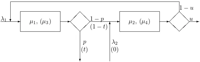
Figure 1.1 provides a picture of the model: there are two stations, each with one exponential server. Each station has its own waiting line, but the line of station 2 is
λ1
p (t)
1−p (1−t)
u 1−u
λ2
(0)
µ1, (µ3) µ2, (µ4)
✲ ✲ ✲ ✲ ✲
❄
✻ ❄
❅❅ ❅ ❅
[image:2.595.107.426.573.672.2]❅❅ ❅ ❅
limited toN−1, including the space for service. Arrivals to the network are Poisson, and the arrival rates areλi for station i, i = 1,2. After the service with station 1
is completed, the customer leaves the network with probabilityp, and he moves to station 2 with probability 1−p. Similarly, a customer finishing at station 2 leaves the network with probabilityu, and proceeds to station 1 with probability 1−u. The service rates areµi for stationi, i= 1,2. However, if server 1 is idle or blocked, she
helps server 2, increasing her service rate toµ4. Similarly, if server 2 is idle, she helps
server 1, bringing her service rate toµ3.
To properly describe the model, we need to state what happens if allN−1 spaces of line 2 are taken. It seems natural to assume that in this case, no arrivals from the outside the network can join line 2. However, some customers finishing line 1 may not leave, but, since line 2 has no space left, they remain in station 1, thereby blocking this station and preventing any service completions. Since this is undesirable, we assume that when the line reachesN −1, the probability of a customer leaving the network changes from pto t, where t > p. It is convenient to consider the customer blocking station 1 as belonging to line 2, which means that line 2 can range from 0 toN.
The outline of the paper is as follows. We first derive the transition matrix of our model, which is a block-structured matrix. We then formulate the corresponding block-structured equilibrium equations. These equations can be classified as either
boundary equations or interior equations. We deal with the interior equations first. They essentially determine whether or not the system is recurrent, a topic addressed in Section 3. We then solve the interior equations in Section 4, and the boundary equations in Section 5. Section 6 provides some numerical considerations. A summary of our procedure is given in Section 7.
2. Mathematical Formulation. The queueing process has two random vari-ables, namely X1 (X1 ≥ 0) and X2 (0 ≤ X2 ≤ N), which are the lengths of
lines 1 and 2, respectively. X1 will be called the level, and X2 the phase. If
πij = P{X1 = i, X2 = j} is the steady-state probability, the main objective of
this paper is to findπij. We assume that the system is recurrent. The condition for
the system to be recurrent will be discussed later.
The transition matrix is partitioned according to levels. Consider first the case whereX1>0. In this case, all rates of the transition matrix increasing the level by 1
are included in the matrixQ1, and all rates decreasing the level by 1 are included in
Q−1. The matrixQ0contains the rates that only affect the phases but not the level,
and it also includes the diagonal elements, which are determined such that the sums across the rows of the entire transition matrix are equal to 0. If X1 = 0, then the
rates leaving the level unchanged are not given by Q0, but by a matrix we callQ00.
this matrix is different fromQ1. Hence, the transition matrix becomes
(2.1) Q=
Q00 Q01 0 0 . . .
Q−1 Q0 Q1 0 . . .
0 Q−1 Q0 Q1 . . .
0 0 Q−1 Q0 . . .
.. . ... ... ... . .. .
Markov Processes with transition matrices of the form given by (2.1) are called Quasi-Birth-Death (QBD) processes.
We now discuss how to obtainQ1,Q0,Q−1,Q00 andQ01. Q1 contains all rates
which increaseX1, provided X1 >0. These rates are given by two events, namely
arrivals from outside and arrivals from the second station. Arrivals from outside occur at a rate ofλ1, and they leave the phase unchanged. As a consequence, the diagonal
ofQ1isλ1. Arrivals from station 2 have a rate of (1−u)µ2unless server 1 is blocked
and helps the second server, causing the rate to increase to (1−u)µ4. These events
decreaseX2, which means the subdiagonal ofQ1is (1−u)µ2, except whenX2=N.
It follows that
Q1=
λ1 0 0 . . . 0
(1−u)µ2 λ1 0 . . . 0
0 (1−u)µ2 λ1 . .. ...
..
. . .. . .. . .. ... 0 0 0 (1−u)µ4 λ1
.
Q01 can be obtained fromQ1 by replacing all instances of µ2 byµ4, indicating that
the first server helps the second one. We look atQ−1 next, which is
Q−1=
pµ3 qµ3 0 . . . 0
0 pµ1 qµ1 . . . 0
..
. . .. ... ... ... ..
. . .. ... tµ1 (1−t)µ1
0 0 . . . 0 0
,
where q = 1−p. To obtain Q−1, note that X1 decreases whenever a service at
station 1 is complete, and this happens at a rate of µ3 if the server of station 2 is
idle (X2 = 0), at a rateµ1 if 0< X2 < N, and at a rate of 0 if server 1 is blocked
(X2 =N). After completing service with server 1, customers leave the system with
probabilitypifX2< N−1, and the phase does not change. With probability 1−p,
the customer joins the line of station 2, and the phase increases by 1. In the first case, we get the diagonal elements pµ3 for X2 = 0, and pµ1 for 0 < X2 < N−1,
and in the second case the superdiagonal elements qµ3 and qµ1. ForX2 = N−1,
adjusted accordingly. A customer completing service at station 1 who does not leave while all spaces of station 2 are taken blocks station 1, meaning thatX2=N.
Q0 has the following form as the reader may verify
Q0=
−(λ1+λ2+µ3) λ2 0 . . . 0
uµ2 −(λ1+λ2+µ1+µ2) λ2 . .. ...
0 uµ2 . .. . .. ...
..
. . .. . .. −(λ1+µ1+µ2) 0
0 . . . uµ4 −(λ1+µ4)
.
Note that when there areN−1 customers in line 2, no customers from the outside are admitted. Hence, the rate of going from phase N−1 to phase N without changing levels is notλ2, but 0.
The matrix Q00 reflects the fact that, when the first server is idle, it helps the
second server. Consequently, the rate of the second server increases toµ4. To convert
Q0 into Q00, one must therefore replace all instances of µ2 byµ4. In addition, the
diagonal changes. Hence
Q00=
−(λ1+λ2) λ2 0 . . . 0
uµ4 −(λ1+µ4+λ2) λ2 . .. ...
0 uµ4 . .. ...
..
. . .. uµ4 −(λ1+µ4) 0
..
. . .. . .. uµ4 −(λ1+µ4)
.
We now have identified all blocks of the matrixQ given in equation (2.1). The row vector of the equilibrium probabilities π can now be found in the normal way by solvingπQ= 0, subject to the condition that the sum of all equilibrium probabilities equals 1. If we partitionπaccording to levels, withπicorresponding to leveli, 0 =πQ
expands to
0 =π0Q00+π1Q−1
(2.2)
0 =π0Q01+π1Q0+π2Q−1
(2.3)
0 =πn−1Q1+πnQ0+πn+1Q−1, n >1.
(2.4)
Equation (2.4) is a difference equation with matrices as coefficients, and their solutions are similar to the standard difference equations. Specifically, one has (see Bertsimas, [3], Mitrani and Chakka [15] and Morse [16]):
(2.5) πn=gxn−1, n≥1,
where g= [g0, g1, . . . , gN] must be different from 0. (We usegxn−1 rather thangxn
because π1=g is more conducive for our purposes thanπ0 =g). Substituting (2.5)
into (2.4) yields
(2.6) 0 =gxn−2
Q1+gxn −1
If we define
Q(x) =Q1+Q0x+Q−1x 2,
then (2.6) implies 0 = gQ(x). The problem is to find the scalarsx and the corre-sponding vectorsg which satisfygQ(x) = 0. In general, this problem is known as the
generalized eigenvalue problem(see [5] for details). The matrixQ(x), or as it is known in literature,Q(λ), is often called aλ-matrix. Generally, anyxsatisfyinggQ(x) = 0 is called a generalized eigenvalue, and the corresponding vector g is a generalized eigenvector. Clearly, a vectorg= 0 exists if and only if detQ(x) = 0. If this equation has multiple roots, then problems arise which are similar to the ones encountered in in standard difference equations with multiple zeros of the characteristic equation. For details, see [5] and [8]. Fortunately, we will show later that ifλ1>0, all eigenvalues
are distinct, and that they are all positive. Hence, we will assume λ1 >0, and that
all eigenvalues are distinct. If the process is recurrent, the eigenvalues are also inside the unit circle. To see this, note that according to Neuts [18, Theorem 1.2.1], there is a matrixRsuch that
πn =π1Rn−1, n≥1.
Here,R is a positive matrix, and its spectral radius is less than 1, which means that allN+ 1 eigenvalues ofRare inside the unit circle. According to Naoumov [17], there is a stochastic matrix Γ, and an invertible matrixY such that
Q(x) = (R−Ix)Y(Γx−I).
It follows that all eigenvalues ofR must also be eigenvalues of Q(x). Therefore, if the process is recurrent, Q(x) hasN + 1 eigenvalues inside the unit circle. This is important because we will need N + 1 solutions to satisfy (2.2) and (2.3) as will be shown later, and solutions with |x| ≥ 1 cannot be used because πn would not
converge. We should also note that according to Perron-Frobenius (see e.g. [2]), the largest eigenvalue ofRis simple and positive, and so is the corresponding eigenvector.
3. Conditions for Recurrence. Before we investigate how to find the equi-librium probabilities, we have to give conditions for their existence, that is, we have to show that the process is positive recurrent. We do this by considering the drift of the process [14]. The drift is defined as the expected increase, or, if negative, the expected decrease of the process, given the boundaries are ignored. If the drift is neg-ative, that is, the process drifts toward level 0, then the process is positive recurrent. If the drift is 0, it is null-recurrent, and if the drift is away from zero, the process is non-recurrent. To find the drift, we first have to find a vector ¯π, which indicates the probabilities of being in the different phases given there are no boundaries. One has
0 = ¯π(Q−1+Q0+Q1).
equal to 1. The process is positive recurrent if and only if this expression is negative. This will now be worked out for our model.
We notice that Q−1 +Q0+Q1 is the incremental generator of a birth-death
process, and we find
¯
πi+1= ¯πiβi/δi+1
where theβi are the birth-rates, that is, the rates on the superdiagonal, and δi are
the death rates, that is, the rates on the subdiagonal. Here β0=qµ3+λ2
βi=qµ1+λ2, i= 1,2, . . . , N−2
βN−1= (1−t)µ1
δi=µ2, i= 1,2, . . . , N−1
δN =µ4.
Fori= 1,2, . . . , N−2,βi is independent ofi, and we can write
(3.1) γ= βi
δi+1
=qµ1+λ2 µ2
.
The sign of the drift is obviously independent of any positive factor of ¯π. Hence, if ¯πi
is theith element of ¯π, we can set ¯π1= 1, and we obtain
¯
π0= µ2
λ2+qµ3
(3.2)
¯
πi=γi−1, i= 1,2, . . . , N−1
(3.3)
¯
πN = (1−t)µ1
µ4
γN−2
. (3.4)
As one can easily verify
(Q1−Q−1)e= [λ1−µ3,(1−u)µ2+λ1−µ1, . . . ,(1−u)µ2+λ1−µ1,(1−u)µ4+λ1] T.
The values of this column vector obviously give the drift for the different states. Multiplying these values with ¯πas given in equations (3.2) to (3.4) yields
(3.5)
µ2(λ1−µ3)
λ2+qµ3 +
((1−u)µ2+λ1−µ1)(1−γN−1)
1−γ +
((1−u)µ4+λ1)(1−t)µ1γN− 2
µ4 , γ = 1
µ2(λ1−µ3)
λ2+qµ3 + (N−1)((1−u)µ2+λ1−µ1) +
((1−u)µ4+λ1)(1−t)µ1
µ4 , γ= 1
This expression must be negative in order for the process to be recurrent.
server 1 once finished with server 2. Mathematically, this meansλ2= 0, p=t= 0,
q= 1 andu= 1. Equation (3.5) then implies:
λ1<
1−γN (1−γ)
1 µ3+
1
µ4γ
N−1
+1
µ2(1
−γN−1)
µ1=µ2 N
1
µ3+ 1
µ4+
N−1
µ
µ1=µ2=µ.
Ifµ4=µ1 andµ3=µ2, that is, if servers do not move, then this result can easily be
converted into the one given by [12].
Remark 1:If the second server has an insufficient capacity to handle the average flow, it is still possible that the first server can help sufficiently to make the problem recurrent. In fact, in this case, the mathematical analysis does not change if instead of blocking, the first server helps the second one as soon as the length of the second server reachesN.
Remark 2: If server 1 can not help while blocked, then none of the matrices Q−1,Q0, orQ1 containµ4. If this is the case, recurrence, or the lack of it, therefore
cannot be affected byµ4. This seems somewhat counterintuitive. The explanation of
this is that no matter how highN is, eventually, server 1 is blocked, and at this point in time, the service rate of server 2 determines the potential throughout. Of course, the higherµ4 andN, the longer it takes the process to become blocked.
4. Difference Equations for the Eigenvectors.
4.1. Direct Solution of the Difference Equations. The equation
gQ(x) =g(Q1+xQ0+x2Q−1) = 0
can be expanded as follows (see [9] and [10]):
0 =−g0((λ1+λ2+µ3)x−λ1−pµ3x2) +g1µ2(ux+ 1−u)
(4.1)
0 =g0(qµ3x2+λ2x)−g1((λ1+λ2+µ1+µ2)x−λ1−pµ1x2)
+g2µ2(ux+ 1−u)
(4.2)
0 =gi−1(qµ1x 2+λ
2x)−gi((λ1+λ2+µ1+µ2)x−λ1−pµ1x2)
+gi+1µ2(ux+ 1−u), i= 2, . . . , N−2
(4.3)
0 =gN−2(qµ1x 2+λ
2x)−gN−1((λ1+µ1+µ2)x−λ1−tµ1x 2)
+gNµ4(ux+ 1−u)
(4.4)
0 =gN−1(µ1(1−t)x 2)
−gN((λ1+µ4)x−λ1).
(4.5)
These equations must be solved forxand forg= [g0, g1, . . . , gN], up to a factor. The
g2, . . . . This leads to the following set of equations, whereβ=u+ (1−u)/x:
g1=λ1+λ2+µ3−λ1/x−pµ3x
µ2β
(4.6)
g2=g1
λ1+λ2+µ1+µ2−λ1/x−pµ1x
µ2β −
qµ3x+λ2
µ2β
(4.7)
gi+1=giλ1+λ2+µ1+µ2−λ1/x−pµ1x
µ2β −gi
−1
qµ1x+λ2
µ2β ,
(4.8)
i= 2, . . . , N−2 gN =gN−1
λ1+µ1+µ2−λ1/x−tµ1x
µ4β −
gN−2
qµ1x+λ2
µ4β
. (4.9)
Equation (4.8) will be called the homogeneous equation, and equations (4.6), (4.7) and (4.9) will be called heterogeneous equations. To express the residual of (4.5) it is convenient to introducegN+1 as follows:
(4.10) gN+1=gNλ1+µ4−λ1/x
µ4β −gN −1
µ1(1−t)x
µ4β .
Clearly,gN+1is a function ofx, and to express this, we will sometimes writegN+1(x).
Every eigenvaluexmust satisfy gN+1(x) = 0, and ifgN+1(x) = 0, (4.10) reduces to
(4.5). We note that ifx= 0, limits arguments must be used. This causes no problem, however, because we will show that all eigenvalues are positive. If x > 0, g0 can
never vanish except for the trivial solution, as the reader may verify. This justifies the choiceg0= 1.
For our algorithms, sign variations will be crucial. We say that the sequence [g0, g1, . . . , gN+1] has a sign variation if gigi+1 <0. Ifgi= 0, a sign variation occurs
ifgi−1gi+1<0,i= 1,2, . . . , N. We denote the number of sign variations for a given
value ofxbyn(x).
Theorem 4.1. If λ1>0, there are exactlyN+ 1 distinct eigenvalues between0
and1. Also, if the valuesx0> x1> . . . > xN, thenn(xi) =i.
Proof. The proof depends on Sturm sequences. For {gi,0 ≤ i ≤ N + 1} to
be a Sturm sequence, we must have g0 > 0, and if gi = 0, gi−1gi+1 < 0. It is
easily verified that both conditions hold as long as x >0. It is not difficult to show that in any Sturm sequence, n(x) cannot change its value unless gN+1 = gN+1(x)
has a single zero. Hence, the number of zeros in the interval (a, b) cannot exceed |n(a)−n(b)|. If x0 is the Perron-Frobenius eigenvalue ofR, thenx0 is positive, and
so is the corresponding eigenvectorg(x0). Hence,n(x0) = 0. On the other hand, if
x= 0+, and λ1 >0, then, by equations (4.1) to (4.4) and (4.10), gi andgi+1 have
opposite signs fori= 0,1, . . . , N. This impliesn(0+) =N+ 1. Hence, there must be N+ 1 eigenvalues between 0 and x0+, and we can denote these eigenvalues by xN,
xN−1, . . . ,x1,x0, with xN < xN−1 < . . . x1< x0. With this convention,n(xi) =i.
This completes the proof. A similar proof can be found in [6, pg. 102].
When λ1 = 0, then the theorem does not apply. In this case, x = 0 is an
λ2
µ1, (µ3) µ2, (µ4)
✲ ✲ ✲ ✲
❄
[image:10.595.136.398.166.267.2]✻ ❄
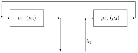
Fig. 4.1.System withλ1=u= 0,p=t= 1.
of a Sturm sequence. In fact, the case where λ1 = 0, u = 0 p = t = 1, µ1 = µ3
and µ2 = µ4 has been analysed in [8]. This system is depicted in Figure 4.1. For
this system, it turned out that⌈N/2⌉(the ceiling ofN/2) eigenvalues are 0, and the remaining ones are in (0,1). Hence, there are now multiple eigenvalues, an issue dealt with in [8].
Theorem 4.1 implies that there cannot be any zeros in the interval (a, b), 0< a < b, if n(a) =n(b). This can be used to exclude intervals from further search. In fact, one can start with an appropriate initial interval, and divide the interval into half, and if one subinterval contains no zeros ofgN+1(x), one can concentrate on the other
half. This results in either one or two subintervals, which can be searched in a similar fashion. This continues until there is a distinct interval for every zero. The following algorithm to find the eigenvaluesxnx2=x[nx2]implements this idea (see [7]):
procedure getx(x1,nx1, x2, nx2) if (nx1=nx2) return
x := (x1+x2)/2 if (x2−x1 ≤ǫ)
then if (nx1 =nx2+1) x[nx2] := x and return else report multiple eigenvalues and return nx := n(x)
getx(x1,nx1, x, nx) getx(x, nx, x2, nx2) return
The initial call to start the algorithm would be getx(a, n(a), b, n(b)) if all zeros of interest are in the interval (a, b). In [7], the gn were found recursively, starting with
g0= 1, and using (4.6) to (4.9). Here, we will give a more efficient algorithm.
4.2. Solution of the Difference Equations. It is well known thatgi =yi−1,
i≥1, is a solution of (4.3). Substitutingyi−1
forgiin (4.3) yields, after simplifications
(4.11) 0 =y2−yλ1+λ2+µ1+µ2−λ1/x−pµ1x
µ2β +
qµ1x+λ2
This quadratic equation has two solutions
(4.12) y1=
b(x)− d(x)
2 , y2=
b(x) + d(x)
2 ,
where
b(x) = λ1+λ2+µ1+µ2−λ1/x−pµ1x
µ2β ,
(4.13)
d(x) =b(x)2−4 qµ
1x+λ2
µ2β
. (4.14)
Ifd(x) = 0, we havey1=y2=y. Also useful are the equations,
(4.15) y1+y2=b(x), y1y2=
qµ1x+λ2
µ2β
.
Becausex >0 andβ =u+ (1−u)/x >0,y1y2>0. Clearly,
(4.16) gn=
d1yn1−1+d2yn2−1 ifd(x)= 0
(d1+ (n−1)d2)yn−1 ifd(x) = 0 n= 1,2, . . . , N−1.
To findd1andd2, we first obtaing1andg2 from (4.6) and (4.7), and we then solve
(4.17) g1=d1+d2, g2=d1y1+d2y2 ifd(x)= 0, g1=d1, g2= (d1+d2)y ifd(x) = 0.
This yields
(4.18)
d1=
g1y2−g2
d(x) , d2=
g2−g1y1
d(x) ifd(x)= 0, d1=g1, d2= g2
y −g1 ifd(x) = 0.
Ifd(x)≥0, we can calculategN−2andgN−1using (4.16), and this allows us to obtain
gN from (4.9) andgN+1 from (4.10). This needs fewer floating point operations than
the recursive calculation suggested by (4.3), and since every floating point operation leads to some rounding error, this also tends to increase the accuracy of the results.
Whend(x)<0,y1andy2are complex conjugate, we use (d, α) and (r, φ) as the
polar coordinates ofd1 andy1, respectively. To fix the sign of the angles, we adhere
to the convention
d1=d(cosα−isinα)
y1=r(cosφ−isinφ).
The expression involving y1, together with (4.12) implies thatφ >0. On the other
on (4.18) shows that the imaginary part ofd1is−g1b(x)/2 −g2 √
−d(x) , and it follows that the
sign ofαis equal to the sign ofg1b(x)−2g2. Moreover
2d=
g2 1+
(2g2−g1b(x))2
−d(x) ,cosα= g1
2d (4.19)
r=
λ2+qµ1x
µ2β
,cosφ=b(x) 2r . (4.20)
With the above notations, one obtains, after a minor calculation (4.21) gn= 2drn−1cos((n−1)φ+α).
4.3. The Location of the Eigenvalues. To locate the eigenvalues, we need the number of sign variationsn(x). To do this, we will need to make use of the sequence {(−1)ng
n, n = 0,1, . . . , N + 1}. Since gn and gn+1 have different signs whenever
(−1)ng
n and (−1)n+1gn+1 have the same sign, the number of sign variations of the
sequence {gn, n = 0,1, . . . , N + 1} equals the number of sign permanences of the
sequence {(−1)ng
n, n = 0,1, . . . , N+ 1} and vice-versa. We also define g(n) to be
given by (4.16), except thatnis real.
We now concentrate on the number of sign variations ofgn forn= 1,2, . . . , N−1.
Ifd(x)>0,y1 andy2 have the same sign because of (4.15) and the fact thatβ >0.
Let us first consider the case wherey1 andy2 are both positive. The equation (4.16)
implies thatgnandgn+1will have different signs only ifg(m) = 0 for somembetween
nandn+ 1. This implies
d1
d2
= y
1
y2
m .
This equation has at most one solution, that is, there is at most one sign variation in the sequence{gn, n= 1,2, . . . , N−1}. Hence, the number of sign variations can be
found as
(4.22) I(g1≤0) +I(g1gN−1<0) +I(gNgN+1<0) +I(gN−1= 0) +I(gN = 0).
Here, I(H) is 1 if the condition H holds, and 0 otherwise. If y1 and y2 are both
negative, we can use the same equation to find the number of sign variations of the sequence {(−1)ng
n, n = 0,1, . . . , N + 1}, except that all gn must be replaced by
(−1)ng
n. If this number is ¯n(x), thenn(x) =N + 1−n(x).¯
Ifd(x) = 0,y1=y2=y=b(x)/2, and sincey1y2= 0,b(x)= 0. Ifb(x)>0, then
yn−1
=b(x)2 n
−1
>0. We defineg(n) according to (4.16) and conclude, using also (4.18) that a sign change can only occur ifg1+ (m−1)(b(x)2g2 −g1) = 0 for some value
It is clear that ify1andy2are both positive,b(x)>0, and ify1 andy2 are both
negative, b(x)<0. The converse also holds, that is, ifb(x)>0, and y1 and y2 are
real, they must both be positive. In this case, (4.22) indicates thatn(x) must be less than or equal to 3+3=6. Similarly, ifb(x)<0,n(x)≥N−2. It follows that there are at most 3 eigenvalues leading to real values for y1 and y2. All other eigenvalues
must correspond to complex values fory1andy2.
To locate the eigenvalues satisfyingd(x)<0, we use the following theorem
Theorem 4.2. The functiond(x)given by(4.14)has exactly2zeros in(0,1), say
x(l) andx(r). In fact, the eigenvalues corresponding to the complex case, d(x) <0, are in the interval(x(l), x(r)).
Proof. We multiplyd(x) by (βµ2)2 to get the following expression
(s−λ1/x−pµ1x)2−4µ2β(qµ1x+λ2),
wheres=λ1+λ2+µ1+µ2. This expression is a polynomial of degree 4, and it can
have at most four zeros. It converges toλ2
1/x2asx→0, and it equals (λ2+qµ1−µ2)2
forx= 1. Since both values are positive and the functiond(x) is continuous on (0,1), the number of zeros must be even in that interval, that is, there are either 0, 2 or 4 zeros ofd(x). However,d(x)<0 ifb(x) = 0, andb(x) has a zero in (0,1) and a zero in [1,∞), which implies thatd(x) has exactly two zeros in (0,1) as claimed. To show thatb(x) has one zero in (0,1) and one zero in [1,∞), consider
(s−λ1/x−pµ1x) =−(pµ1x2−sx+λ1)/x.
Ifx1andx2are the 2 zeros ofb(x),x1x2=λ1/(pµ1)>0, that is,x1andx2must have
the same sign. Moreover,b(x)<0 as x→0, and b(1)>0. Hence,b(x) has exactly one zero in (0,1), which means that the other one must be outside the interval. Since x1x2 >0, the zero outside (0,1) must be positive, that is, 0 < x1 <1 < x2. This
completes the proof that d(x) has exactly two zeros in (0,1), whereas the other two zeros are in [1,∞).
For the cased(x)<0, the number of sign changes is given by n(x) =I(g1<0) +
(N
−2)φ+α+ 1/2 π
−
α+ 1/2 π
+ 1 +I(gN−1gN <0) +I(gNgN+1<0) +I(gN = 0) +I(gN+1= 0).
(4.23)
As before,I(·) is the indicator function,⌊x⌋is the floor ofx, and⌈x⌉the ceiling. To prove (4.23), we have to find the number of sign variations between g1 and
gN−1. To do this, we defineg(n) to be the continuous version of (4.21). Clearly,g(n)
is zero whenever (n−1)φ+αis equal to (k+ 1/2)π, wherekis an integer. Sincen ranges from 1 toN−1, this means
α+ 1/2
π ≤k≤
α+ (N−2)φ+ 1/2
π .
Sincekis integer, this implies
α+ 1/2 π
≤k≤
α+ (N−2)φ+ 1/2 π
The number of distinct values ofk within these bounds equals
α+ (N−2)φ+ 1/2 π
−
α+ 1/2 π
+ 1.
The proof of (4.23) can now be completed by counting the sign variations outside the interval in question. Note that if either g1 = 0 or gN−1 = 0, this is counted as a
sign variation betweeng1 andgN−1. Also note that sinceφ < π, every zero ofg(n)
corresponds to a sign change.
We now can apply the procedure “getx” as follows. First, we calculate x(l) and x(r), and we find n(x(l)) and n(x(r)). We also find g
N+1(x(l)) to see if x(l) is an
eigenvalue, and we do the same for gN+1(x(r)). After this, the interval from 0 to 1
is divided into three subintervals, namely (0, x(l)), (x(l), x(r)) and (x(r),1), and the
procedure “getx” is applied for each interval.
5. The Boundary Equations. Due to the fact thatQ01=Q1, the treatment
of the boundary equations in this model is different from the one in [9] or [10]. We first solve (2.2) forπ0, which yields
(5.1) π0=π1Q−1(−Q00) −1
.
It follows from the theory of Markov chains that if the process is recurrent,Q00 has
an inverse. We now substitute (5.1) into (2.3) to obtain (5.2) 0 =π1(Q0+Q−1(−Q00)
−1
Q01) +π2Q−1=π1Q¯11+π2Q−1,
where ¯Q11= (Q0+Q−1(−Q00) −1
Q01). We now have to combine the solutions given
by (2.5) to satisfy this equation.
For each eigenvalue xν, ν = 0,1, . . . , N, the eigenvectorg(ν) is given by solving
(4.6) to (4.9). Any solution πn = g(ν)xnν−1 solves (2.4), and so does any linear
combination of these solutions. In other words, all possible solutions have the form
(5.3) πn=
N
ν=0
cνg(ν)xn −1
ν , n >0.
To write this equation in matrix form, let Λ = diag(xν), and letGbe the (N+ 1)×
(N + 1) matrix [g(0), . . . , g(N)]T, where T denotes the transpose. Therefore, (5.3)
becomes:
(5.4) πn =cΛn−1G.
We need to determinec= [c0, c1, . . . , cn] in such a way that (5.2) is satisfied. Clearly,
π1=cG, π2=cΛG.
Hence (5.2) leads to
On the other hand, using (5.1) and the fact that the sum of all probabilities must be one, we have
1 = (π0+ ∞
n=1
πn)e=c
GQ−1(−Q00) −1
+
∞
n=1
Λn−1
G
e
=c
GQ−1(−Q00) −1
+ diag( 1 1−xn)G
e. (5.6)
Here,eis a column vector with all entries equal to 1. Equations (5.5) and (5.6) fully determine c. When solving (5.5), we can express all ci as a multiple of c0, and use
(5.6) to findc0. Notice that c0 is the coefficient of the dominant eigenvalue x0, and
it must be non-zero.
6. Numerical Considerations. It has been shown in [7] that given a certain precision 2−α
, all eigenvalues can be found by evaluating gN+1(x) for (N + 1)(α−
log2(N+ 1)) + log2(N+ 1) different values of x. Since the number of operations to evaluategN+1(x) is independent ofN, the time complexity of finding all eigenvalues
is essentially O(Nlog2N), which is very satisfactory. One can even improve upon
this by using the secant method or other root finding methods once one hasN + 1 intervals, each containing exactly one eigenvalue.
The question arises as to what extent rounding errors affect the results. To get a handle on this question, let us compare our method with the method of Neuts [18]. There,R is determined by using the following matrix equation
(6.1) 0 =Q1+RQ0+R2Q−1.
We can assume that even if a fast method is used, such as suggested in [13], this equation is only met at a precision of ±ǫ, where ǫ is some multiple of the machine precision. In our case, we solve
(6.2) 0 =g(i)(Q1+xiQ0+x2iQ−1), i= 0,1, . . . , N.
As in the case of (6.1), we concentrate on the residuals. This makes the analysis quite different from the analysis concentrating on the errors of the vectorsg(i). The
difference is that when calculating thegj(i)using (4.6) to (4.10), errors in the values of gj(i)for lowjoften have a catastrophic effect on thegj(i)for higher values ofjbecause they are increased due to subtractive cancellation. The residuals, on the other hand, are independent of what happens earlier in the recursion, as pointed out in [7]. In fact, no matter what values of gi−1 and gi is used, gi+1 is always determined such
that the residual is zero except for rounding. Hence, earlier errors have no influence on the present residual. This means that except for the last equation, the residuals of (6.2) can be expected to be small. The residuals of the last equation, of course, are essentially given by gN+1, and we make this residual small by choosing the correct
value ofx. Hence, (6.2) will be satisfied rather accurately. Once allg(i) andx
i are found, one calculates
πn = N
i=0
Table 6.1
The maximum value of|ci|for selected problems
µ1=µ2= 10,µ3=µ4= 20
N λ |ci|max
5 8 0.0292 10 8 0.0203 15 8 0.0090 20 8 0.0349 5 9 0.0169 10 9 0.0127 15 9 0.0112 20 9 0.0765
It is obvious that if all |ci| ≤ 1, then the resulting πn is again correct with a high
precision. What is possible, however, is that some ci have high values, and in this
case, any errors are multiplied by a large number. Hence, large values of |ci| are
an indication of potential problems. We therefore calculated the ci for a number of
models, and obtained the largest absolute value ofci, which we denote by|ci|max. The
results are given in Table 1. The model is the standard model, with every customer going from line 1 to line 2, no premature departures, and no feedback. The values of µi,i= 1,2,3,4 are as indicated in Table 1. As one can see, theciare rather small, and
they increase only slightly asN increases. Hence, the residuals of (6.2) remain small. We also note that ifπn is calculated for high values ofn, only the Perron-Frobenius
eigenpair (x0, g(0)) and the correspondingc0 matters. A little reflection shows that
this guarantees a small relative error for high values ofn.
We note that our method is already advantageous for N = 20 as compared to matrix analytic methods. In matrix analytic methods, matrix multiplications are required in each iteration, and a single matrix multiplication requires 2N3operations,
which makes 16000 operations forN = 20. This has to be compared withNlog2N
for our method, which is around 100 for the same value ofN.
7. Summary. To solve the equationgQ(x) = 0, we choose some value forxand determine the vectorsg such that only the last entry of the row vectorgQ(x) differs from zero. This can be done by the following algorithm:
Algorithm
1. Setg0= 1 and findg1 by (4.6) andg2 by (4.7).
2. Findy1 andy2 using (4.12).
3. Findd1 andd2by (4.18).
4. To determinegN−2and gN−1, use (4.16). Ifd(x)<0, (4.21) can be used.
5. Finally, getgN by (4.9) andgN+1by (4.10).
A search procedure is then used to reducegN+1to zero. By using Sturm sequences, we
when the second line reaches its limit. In fact, the method suggested here can be used for any queueing problem leading to a tridiagonal matrixQ(x), such as the bilingual call centre problem studied in [20]. The reason generalizations become easy is that the recursive equations are used directly, and not solved as in [10] and [9].
Notice that the step involving finding all eigenvalues isO(N), and this is the only process that has to be done iteratively. The step involving finding thegi is O(N2),
and finding cby solving (5.5) is O(N3). Hence, the main effort is likely to be spent
findingc, and not finding eigenvectors and eigenvalues.
The equations (4.1) to (4.4) are all satisfied exactly, no matter how accurate or inaccurate the eigenvaluexin question may be. Ifxis not accurate, of course, (4.5) is not satisfied. If (4.1) to (4.5) are satisfied, so are the equilibrium equations for this particular solution. To satisfy the initial conditions, one has to combine these solutions, and unless there are some huge values ci, this combination of solutions
has an accuracy which is comparable to the individual solutions. In fact, one can approximate the accuracy of the final solution by first calculating the residuals of (4.5), sayri is the residual for eigenvectorg(i), and formNi=0|ciri|. In all cases we
considered, this sum turned out to be small.
We should mention that irregular bounds in QBD processes cause difficulties. For matrix-analytic methods, these difficulties are outlined by Neuts [18, pgs. 24-27]. Though we do not use matrix-analytic methods here, we still would have the same problems as Neuts, and our earlier efforts were considerably hampered because of this difficulty. In this paper, as in [7], we simply bypass this problem by reducing the transition matrix to one that has a regular boundary.
Although in this paper we restricted the second queue to be finite, we believe that this paper may contain a method leading to the solution for two infinite queues. In this case, there is of course no blocking. We are hoping to solve this problem in a not too distant future.
Acknowledgments. This research was supported by the Natural Sciences and En-gineering Research Council of Canada. We also thank the referees for their useful comments.
REFERENCES
[1] S. Andradottir, H. Ayhan, and D. Down. Server assignment policies for maximizing the steady-state throughput of finite steady-state queueing system.Management Science, 47:1421–1439, 2001. [2] A. Berman and R. J. Plemmons.Nonnegative Matrices in the Mathematical Sciences. Academic
Press, New York, 1979.
[3] D. Bertsimas. An analytic approach to a general class of G/G/s queueing systems.Operations Research, 38:139–155, 1990.
[4] D. P. Bischak. Performance of a manufacturing module with moving workers.IIETransactions, 28:723–733, 1996.
[5] I. Gohberg, P. Lancaster, and L. Rodman.Matrix Polynomials. Academic Press, New York, 1982.
[6] W. K. Grassmann. Real eigenvalues of certain tridiagonal matrix polynomials, with queuing applications.Linear Algebra and its Applications, 342:93–106, 2002.
Marko-vian two-dimensionalqueueing problems.INFORMS Journal on Computing, 15:412–421, 2003.
[8] W. K. Grassmann. Finding equilibrium probabilities of qbd processes by spectral methods when eigenvalues vanish.Linear Algebra and its Applications, 386:207–223, 2004. [9] W. K. Grassmann and S. Drekic. An analytical solution for a tandem queue with blocking.
Queueing systems: Theory and Applications, 36:221–235, 2000.
[10] W. K. Grassmann and J. Tavakoli. A tandem queue with a movable server: An eigenvalue approach.SIAM Journal on Matrix Analysis and Applications, 24:465–474, 2002. [11] B. R. Haverkort and A. Ost. Steady-state analysis of infinite stochastic Petri nets: A
com-parison between the spectralexpansion and the matrix-geometric method. in Proc. 7th International Workshop on Petri Nets and Performance Models, Saint Malo, France, 1997, IEEE Computer Society Press, pp. 36–45.
[12] A. G. Konheim and M. Reiser. Finite capacity queueing systems with applications in computer modeling.SIAM Journal on Computing, 7:10–229, 1978.
[13] G. Latouche and V. Ramaswami. A logarithmic reduction algorithm for quasi-birth-death pro-cesses.Journal of Applied Probability, 30:650–674, 1993.
[14] G. Latouche and V. Ramaswami.Introduction to Matrix Analytic Methods in Stochastic Mod-eling. ASA-SIAM Series on Applied Probability, SIAM, Philadelphia, 1999.
[15] I. Mitrani and R. Chakka. Spectral expansion solution for a class of Markov models: Application and comparison with the matrix-geometric method.Performance Evaluation, 23:241–260, 1995.
[16] P. M. Morse.Queues, Inventories and Maintenance. John Wil ey, New York, 1958.
[17] V. Naoumov. Matrix-multiplicative approach to quasi-birth-and-death processes analysis. in Matrix-Analytic Methods in Stochastic Models, Marcel Dekker, New York, 1996, pp. 87– 106.
[18] M. F. Neuts. Matrix-Geometric Solutions in Stochastic Models. Johns Hopkins University Press, Baltimore, 1981.
[19] M. F. Neuts.Structured Stochastic Matrices of M/G/1 Type and Their Applications. Marcel Dekker, New York, 1989.
[20] D. A. Stanford and W. K. Grassmann. Bilingual server call centres. in Analysis of Commu-nication Networks: Call Centres, Traffic and Performance, D. R. McDonald and S. R. E. Turner, eds.,Fields Institute Communications, The American MathematicalSociety, 2000, pp. 31–47.