Modeling the effects of health on economic growth
Alok Bhargava
a,∗, Dean T. Jamison
b,
Lawrence J. Lau
c, Christopher J.L. Murray
daDepartment of Economics, University of Houston, Houston, TX 77204-5882, USA bCenter for Pacific Rim Studies, University of California, Los Angeles, CA, USA
cDepartment of Economics, Stanford University, Stanford, CA, USA dDepartment of International Health, Harvard School of Public Health,
Boston, and World Health Organization, Geneva, Switzerland
Received 1 February 2000; received in revised form 1 January 2001; accepted 11 January 2001
Abstract
This paper investigates the effects of health indicators such as adult survival rates (ASR) on GDP growth rates at 5-year intervals in several countries. Panel data were analyzed on GDP series based on purchasing power adjustments and on exchange rates. First, we developed a framework for modeling the inter-relationships between GDP growth rates and explanatory variables by re-examining the life expectancy–income relationship. Second, models for growth rates were estimated taking into account the interaction between ASR and lagged GDP level; issues of endogeneity and reverse causality were addressed. Lastly, we computed confidence intervals for the effect of ASR on growth rate and applied a test for parameter stability. The results showed positive effects of ASR on GDP growth rates in low-income countries. © 2001 Elsevier Science B.V. All rights reserved.
JEL classification:C22; C33; E17; F43; I12; O11; O47
Keywords:Economic development; Economic growth; Health; Random effects models; Panel data; Simultaneity
1. Introduction
The 20th century has seen remarkable gains in health. Average life expectancy in devel-oping countries was only 40 years in 1950 but had increased to 63 years by 1990 (World Bank, 1993). Factors such as improved nutrition, better sanitation, innovations in medical technologies, and public health infrastructure have gradually increased the human life span. The relative contribution of these factors depends on the level of economic development; there are synergisms between the underlying factors operating in complex ways. Thus, for
∗Corresponding author. Tel.:+1-713-743-3837; fax:+1-713-743-3798.
E-mail address:[email protected] (A. Bhargava).
example, while recognizing various determinants of life expectancy, Preston (1976) empha-sized economic development as the most important factor. However, since life expectancy is strongly influenced by child mortality, low-cost interventions such as the provision of ante natal care and vaccination programs in poor countries can be effective instruments for raising life expectancy. More generally, economic development depends on the level of skills acquired by the population and on capital formation. The former is influenced by child nutrition, educational infrastructure, and households’ resources, including parents’ physical health and cognitive attainment (e.g. Fogel, 1994; Scrimshaw, 1996; Bhargava, 1998, 1999). Capital accumulation depends on the savings rate that is also influenced by adult health.
Analyses of the inter-relationships between health and economic productivity can be conducted at the individual level, at regional levels within a country, and for aggregate data on countries. In developing countries, there are numerous micro studies in biological and social sciences showing benefits of better health on productivity (e.g. Basta et al., 1979; Spurr, 1983; Bhargava, 1997; Strauss and Thomas, 1998). Quantifying the relationship between health indicators and economic productivity is more subtle in developed countries. For example, the effects of disability on employment status have been investigated in The Netherlands (Stronks et al., 1997); the relationship was stronger in physically demanding occupations where earnings are typically low. The earnings of a large proportion of the population, however, depend on their general health and well-being, including mental health. While psychologists have investigated the decline with age in components of cognitive abilities (Horn and Hofer, 1992), the effects of such factors on individuals’ productivity remain largely unknown.
Recently, aggregate data at the country level for the post-war period have become acces-sible (Penn world table (PWT), Summers and Heston, 1991; world development indicators (WDI), World Bank, 1998). Panel data on countries have been extensively used to elucidate economic relationships (e.g. Barro and Sala-i-Martin, 1995; Barro, 1997). Because many countries have experienced demographic and health transition in this period, studies can yield insights into the sources of economic growth. The quality of the data, however, can be poor especially in less developed countries, where many of the variables are ‘projections’ from statistical models. For example, the purchasing power parity indices commonly used for constructing the real GDP series in the PWT are based on the information on a subset of 68 countries. Further, most countries face different socio-economic and infrastructural constraints that are difficult to approximate in the analyses. Pooling data across countries can lead to spurious results, especially if the investigators fail to address stochastic proper-ties of the dependent variable in econometric modeling (Sargan, 1964). Such problems are exacerbated in models explaining aggregate variables such as the GDP. Moreover, growth rates averaged over long time periods (e.g. 25 years) tend to describe economic activity in a way that is similar to the GDP. By contrast, the 5-year average growth rates analyzed in this paper show considerable variation but are less noisy than the annual growth rates.
the data used in the analysis. The analytical framework for modeling the effects of health on economic growth is developed in Section 3.1. The econometric framework is outlined in Section 3.2. Issues of possible reverse causality from higher growth rates to the adult survival rates (ASR) are discussed in Section 3.3. A Wald type statistic for the stability of model parameters outside the sample period is developed in Section 3.4. In Section 4.1, average growth rates at 5-year intervals are modeled using a model similar to Barro (1997), but allowing for simultaneity and interactions between some regressors. Instrumental variables estimation methods were used and certain maintained hypotheses were tested (Bhargava, 1991a). In Section 4.2, we elaborate on the role of the interaction between lagged ASR and GDP from a policy standpoint. Stability of the estimated parameters is tested in Section 4.3 by a Wald test using out-of-sample observations for 1995 on GDP from the WDI. The conclusions and the need for collecting additional health statistics are discussed in Section 5.
2. The data
The data used in the analysis were primarily from the PWT (Summers and Heston, 1991) and the WDI (World Bank, 1998). The GDP series in the PWT are in “1985 international dollars” that were based on purchasing power parities for a subset of countries; the GDP series from the WDI was based on the official exchange rates using 1987 constant dollars. The WDI GDP series is likely to show greater variability, because exchange rate fluctuations can induce distortions especially for small countries. However, the PWT GDP series involves estimation of the purchasing power parity indices for countries where the data were not available (Summers and Heston, 1991; Ahmad, 1992). Conclusion from our analysis will be strengthened if GDP series based on purchasing power parities and exchange rates yield similar results.
The total fertility rate, life expectancy, and population variables were available in the PWT and WDI data sets. In addition to life expectancy, we used the ASR (probability of surviving the 60th birthday after reaching the age 15 years; mean=0.702, S.D.=0.14) from Bos (1998). The ASR is less sensitive to child mortality rates and was constructed from World Bank demographic files containing mortality data on countries; figures for some countries were projections from demographic models. Typically, data on total fertility rate and ASR were compiled at irregular intervals. To reduce the effects of projections on the empirical results, we analyzed panel data that were separated by 5-year intervals, i.e. six time observations on the countries (in 1965, 1970, 1975, 1980, 1985, 1990) were used (first observation in WDI series was for 1966).
The education series (average years of education for population aged 15–60) for the six time periods were taken from Barro and Lee (1996). Data on geographical variables such as the area in the tropics, if the country is ‘land-locked’, and an index of openness to trade were from Gallup and Sachs (1998). Overall, the GDP data covered 125 countries in the PWT and 107 countries in the WDI. However, because of missing observations on explanatory variables, the sample sizes used in the estimation were lower for the models for GDP growth rates.
Collins and Bosworth (1996) and Nehru and Dhareshwar (1993) have imputed the data on physical capital for a larger number of countries under certain assumptions on depreciation rates. Because these assumptions are non-standard and because the focus of our analysis was on the relationship between health indicators and economic growth, we do not report the results for aggregate production functions in this paper.
3. A framework for modeling the effects of health on economic activity
3.1. The conceptual framework
Preston (1976) analyzed cross-country data on life expectancy and national incomes for the approximate periods 1900, 1930, 1960 and observed that the curves showed an upward shift over time. For a given income level, life expectancy was highest in 1960s. Moreover, per capita GDP above $600 (in 1963 prices) had little impact in raising the highest life expectancy (73 years) in the 1960s. While recognizing that shifts in the curves had multiple causes, Preston attributed approximately 15% of the gains in life expectancy to income growth, but was less optimistic about the role played by nutrition and literacy. However, recent analyses of historical data suggest larger benefits from improved nutrition (Floud et al., 1991; Fogel, 1994). Furthermore, public health programs reducing sicknesses have beneficial effects on health by preventing the loss of vital nutrients due to infection (Scrimshaw et al., 1959).
Life expectancy (or ASR) in a country is a broad measure of population health, though it need not accurately reflect the productivity of the labor force. For example, suppose that due to poor childhood nutrition, ability of individuals to perform productive tasks diminishes at an early age but, because of access to medical care, life expectancy is high (e.g. the Indian state of Kerala; International Institute of Population Sciences, 1995). Then productivity loss will be under-estimated if life expectancy was used as the sole indicator of health. Indices measuring disabilities of the working population in various occupations would be insightful for assessing productivity loss (e.g. Murray and Lopez, 1996).
At a general level, capital formation requires that a high proportion of the skilled labor force remains active for a number of years; experience is important for technical innovations that take years of investments in research and development. Because detailed information on such variables cannot be utilized in national comparisons, a broader view of health is helpful for interpreting the results. In particular, investments in education and training critically depend on survival probabilities; expenditure on children’s education may be influenced by parents’ subjective probabilities of child survival. All these factors are potentially important for explaining economic growth (e.g. Bloom and Canning, 2000).
prospered during the sample period (1965–1990), while others have not, a model for the proximate determinants of economic growth can shed light on these issues.
The dependence of life expectancy on incomes up until a certain threshold suggests that it would be useful to model the GDP or growth rates using a flexible production function such as the trans-logarithmic function (Christensen et al., 1973; Sargan, 1971). Boskin and Lau (1992) estimated aggregated production functions for five developed countries using annual observations for the post-war period. Kim and Lau (1994) extended the analysis to cover four countries in the Pacific basin where good data on the physical capital stock were available. From the standpoint of modeling the effects of health on economic growth, the flexible functional form approach underscores the interaction between explanatory variables and the importance of squared terms in the model. While precise estimation of coefficients of high order terms would require large sample sizes, the work by Preston (1976) demonstrated the asymmetry in the life expectancy–incomes relationship. It is therefore likely that the impact of health indicators such as ASR on growth rates would depend on the level of GDP. Thus, ASR should be important for explaining economic growth at low levels of GDP. In more affluent settings, investments in education and training, and measures of health such as the decline in cognitive abilities with age, and age-specific disease prevalence rates, may be of greater importance.
3.2. The econometric framework for estimation of static random effects models containing endogenous regressors
The methodology used for the estimation of static random effects models for GDP growth rates in situations where some of the explanatory variables are endogenous was developed by Bhargava (1991a). Let the model be given by
yit =
wherez is time invariant variables,x1 andx2, respectively, exogenous and endogenous time varying variables, andNthe number of countries that are observed inTtime periods. The slope coefficients are denoted by Greek letters. In the models estimated for GDP growth rates, for example, the proportion of area of a country in the tropics is a time invariant explanatory variable. Time varying regressors consist of (lagged) total fertility rate, investment/GDP ratio, ASR, interaction between ASR and GDP, and GDP.
It is important to distinguish between two sets of assumptions for the potential endo-geneity of the time varying variablex2. First,x2may be correlated with the errorsuit in a
general way, i.e.x2are ‘fully’ endogenous variables. Thus,x2j t must be treated as different
variables in each time period. LetX1andX2be, respectively, then1×1 andn2×1 vectors containing the exogenous and endogenous time varying variables (n1+n2=n), and letZ be them×1 vector of time invariant variables. We can write a reduced form equations for the fully endogenous variablesX2as
X2it=
T
j=1
whereFtj(t =1, . . . , T;j =1, . . . , T) andFt∗(t =1, . . . , T) are, respectively,n2×n1
andn2×mmatrices of reduced form coefficients;U2it then2×1 vector of errors. The reduced form Eq. (2) is a general formulation for correlation between the time vary-ing endogenous variables and errorsuit affecting model (1). Thus, for example, lagged
GDP has often been included as an explanatory variable in models for growth rates (Barro and Sala-i-Martin, 1995; Barro, 1997). Caselli et al. (1996) have stressed that lagged GDP should be treated as endogenous. Because the error terms affecting Eq. (1) may have a complex structure (Sala-i-Martin, 1996), it is appealing to treat lagged GDP as a fully en-dogenous variable in the estimation. Similarly, one might postulate that the investment/GDP ratio is a fully endogenous variable; transitory components ofuit may be correlated with
short-term fluctuations in the investment/GDP ratio. Moreover, one can test the hypothe-ses that GDP and the investment/GDP ratio are exogenous variables using sequential procedures.
As noted in Section 2, variables such as ASR and total fertility rate are typically compiled in a country at a certain points of time; the yearly values tabulated in PWT and WDI are often projections from simple statistical models. Extrapolation of a variable such as ASR implies that it cannot be treated as a fully endogenous variable; the time observations on ASR are likely to be systematically related. This will violate the rank condition for parameter identification in models where ASR is assumed to be a fully endogenous variable.
An alternative assumption for endogeneity of variables such as ASR is to assume that only the country-specific random effectsδi are correlated withx2ij t.
x2ijt=λtδi+x2∗ijt (3)
wherex∗
2ijtare non-correlated withδi, andδi are randomly distributed variables with zero
mean and finite variance. This correlation pattern was invoked by Bhargava and Sargan (1983) and is in the spirit of the commonly used random effects models. Endogenous variables represented by Eq. (3) have sometimes been referred to as ‘special’ endogenous variables (Bhargava, 1991b). While Eq. (3) may seem to be a restrictive formulation, it allows countries to possess unobserved ‘permanent’ characteristics that in turn could influence the levels of explanatory variables. For example, countries with high saving rates may invest greater resources in health and education sectors. This will cause the errors on the model for growth rates to be correlated with variables such as the education levels attained by the population. Furthermore, such assumptions are implicit in random effects models that decompose the errorsuit as
uit=δi+vit (4)
wherevitare independently distributed random variables with zero mean and finite variance.
Eq. (4) is a special case of the general formulation for the errors on model (1), which only assumes that the variance covariance matrix ofuit is positive definite.
The main advantage in assuming the correlation pattern (3) is that deviations of thex2ij t
from their time means.
where can be used as [(T −1)n2] additional instrumental variables to facilitate parameter identi-fication and estimation (Bhargava and Sargan, 1983). An efficient three-stage least squares type instrumental variables estimator will be used to estimate Eq. (1), assuming the two types of correlation patterns forx2j t given by Eqs. (2) and (3), and without restricting the
variance covariance matrix ofuit.
Further, in contrast to ordinary time series case, where mis-specification tests have been applied to test the overidentifying restrictions (Sargan, 1958), it is possible to test the validity of exogeneity assumption for explanatory variables in the panel data framework. As shown in Bhargava (1991a), one can sequentially test exogeneity assumptions using statistics based on instrumental variables estimates, because the correlation pattern for special endogenous variables in Eq. (3) is nested within the general formulation (2), where thex2are fully endogenous. The sequential Chi-square test for exogeneity would first test the validity of the special correlation pattern (3). Ifn2time varying variables are postulated to be endogenous, then under the null hypothesis, the first test statistic is asymptotically distributed (for largeNand fixedT) as a Chi-square variable with [T (T −1)n2] d.f. If the null hypothesis cannot be rejected, then we can further test if the time means ofx2given by Eq. (6) are non-correlated with the random effectsδi. The test statistic for the second set
of hypotheses is asymptotically distributed as a Chi-square withTn2d.f. (for details, see Bhargava, 1991a). The overall size of sequential tests can be based on several considerations (e.g. Anderson, 1971; Sargan, 1980).
To summarize the modeling strategy used in the analysis, we proceed by assuming that lagged GDP is a fully endogenous variable and estimate the parameters using an efficient instrumental variables estimator. It is likely that the exogeneity null hypothesis will be rejected for the lagged GDP variable. We can also test whether lagged investment/GDP ratio should be treated as a fully endogenous variable. Due to the potentially low predictive power of the instrumental variables in explaining the endogenous variables in panel data models (Bhargava and Sargan, 1983, p. 1654), we also report the adjustedR-squared for the reduced form equations for lagged GDP in each of the five time periods.
Further, because of extrapolation of variables such as ASR, it would be inappropriate to formulate that ASR and the interaction between ASR and GDP are fully endogenous variables. Instead, we treat these regressors as special endogenous variables as in Eq. (3) and test if their time means given by Eq. (6) are non-correlated with the country specific random effectsδi. We recognize that it would be desirable to use additional time varying
3.3. A formulation for investigating reverse causality from GDP growth rates to adult survival rates
As noted in Section 3.1, Preston (1976) emphasized the likely effects of GDPlevelon life expectancy using cross-country data. By contrast, the recent literature explains GDP growth rates using lagged life expectancy as an explanatory variable. It is therefore important not only to treat lagged GDP level as a fully endogenous variable in model (1), but also to investigate possible reverse causation, i.e. if higher GDP growth rates in the previous period may be the ‘cause’ of higher ASR. Such an investigation would be in the spirit of Fisher (1973). Cochrane (1965) and Cox (1992) discuss certain aspects of interpreting associations in observational data as causal effects.
While one can apply the approach commonly used in time series analysis for testing the significance of lagged values of ASR in the model for GDP growth rate to investigate reverse causality, this procedure would suffer from certain drawbacks. First, as noted above, ASR is based on demographic data collected at a few points in time and the remaining values are projections; the lagged values of a slowly evolving variable such as ASR will be highly correlated with current values. Second, ASR may be correlated with the country specific random effectsδi in model (1) for growth rates thereby making it more likely that the
coefficients of lagged ASR will be significantly different from zero. Third, because our sample size consists of six time observations at 5-year intervals and some explanatory variables are endogenous, the purely time series approach is perhaps unappealing.
The approach used in our analysis is based on developing a model for ASR and investi-gating whether lagged GDP growth rates are significant predictors of ASR, after controlling for many confounding factors. Because the relationship between life expectancy and GDP levelis well-established, we include lagged GDP level as an explanatory variable in the model for ASR and expect it to be a significant predictor. However, this need not be true for lagged GDP growth rates. In the spirit of the discussion in Section 3.1, we also include an interaction term between lagged GDP level and growth rates. Thus, if the coefficient of lagged GDP growth rates is a significant predictor of current ASR, and ASR is also a sig-nificant predictor of growth rates in model (1), then causality could run in either direction, i.e. from GDP growth rates to ASR or from ASR to GDP growth rates. By contrast, if the coefficient of GDP growth rates is not statistically significant in the model for ASR, then causality is more likely to run from ASR to GDP growth rates. Because of the panel nature of the data, we can tackle some of the issues of simultaneity in the estimation of models for GDP growth rates and ASR.
3.4. A Wald type test for parameter stability outside the sample period
of the unknown coefficients in Eq. (1) and letb∗be the corresponding estimates from the cross-section regression for time period (T +1). Then, defining the variance covariance matrix ofb∗byV(b∗,b∗), the Wald statistic for parameter stability is given by
W =(b∗−b)′=[V (b∗, b∗)]−1(b∗−b) (7) Under the null hypothesis of parameter stability, W is distributed (for large N) as a Chi-square variable withkd.f.
4. Empirical results
4.1. Empirical results for models for GDP growth rates
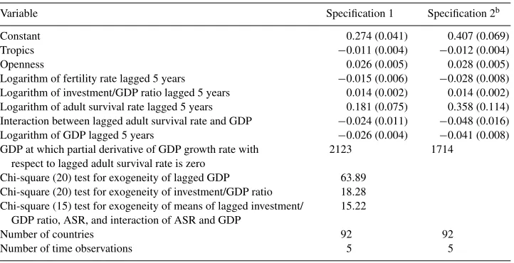
Table 1 presents the empirical results for GDP growth rates for 92 countries at 5-year in-tervals using the PWT GDP series; the stochastic properties of the GDP series are discussed in Bhargava (2000), where it was found preferable to model growth rates. The model is similar in spirit to Barro (1997) but, as will be apparent from the discussion, it differs in a number of important respects. Specification 1 treats the explanatory variables as exogenous; the lagged GDP was a fully endogenous variable in specification 2. The estimation method used for specification 2 was also applied under the additional assumption that lagged in-vestment/GDP ratio was a fully endogenous variable. However, the appropriate Chi-square statistic reported in Table 1 accepted the exogeneity null hypothesis for investment/GDP
Table 1
Estimated slope coefficients from static random effects models for real per capita GDP growth rates 1965–1990 at 5-year intervals using data from PWTa
Variable Specification 1 Specification 2b
Constant 0.274 (0.041) 0.407 (0.069)
Tropics −0.011 (0.004) −0.012 (0.004)
Openness 0.026 (0.005) 0.028 (0.005)
Logarithm of fertility rate lagged 5 years −0.015 (0.006) −0.028 (0.008) Logarithm of investment/GDP ratio lagged 5 years 0.014 (0.002) 0.014 (0.002) Logarithm of adult survival rate lagged 5 years 0.181 (0.075) 0.358 (0.114) Interaction between lagged adult survival rate and GDP −0.024 (0.011) −0.048 (0.016) Logarithm of GDP lagged 5 years −0.026 (0.004) −0.041 (0.008) GDP at which partial derivative of GDP growth rate with
respect to lagged adult survival rate is zero
2123 1714
Chi-square (20) test for exogeneity of lagged GDP 63.89 Chi-square (20) test for exogeneity of investment/GDP ratio 18.28 Chi-square (15) test for exogeneity of means of lagged investment/
GDP ratio, ASR, and interaction of ASR and GDP
15.22
Number of countries 92 92
Number of time observations 5 5
aAsymptotic standard errors are in parentheses.
ratio, conditional on the treatment of lagged GDP as a fully endogenous variable. Next, the investment/GDP ratio, ASR and interaction between ASR and GDP were treated as special endogenous variables, i.e. correlated with the country specific random effectsδi. Another
Chi-square statistic reported in Table 1 accepted the exogeneity null hypothesis, conditional on the treatment of lagged GDP as a fully endogenous variable. The variance covariance matrix of the errors was unrestricted in the estimation and testing procedures.
The main results can be summarized as follows.
1. The coefficient of the percentage of area of a country in the tropics was estimated with a negative sign that was statistically significant. Openness of the economy was positively associated with growth rates; the magnitude of the coefficient was robust to the use of alternative definition of openness in the PWT. The log of total fertility rate was negatively associated with GDP growth rates and was statistically significant. High fertility rates are common in developing countries and increase the demand on resources for health care and education; the work force does not increase equi-proportionately with the pop-ulation. Also, high fertility rates in developing countries often reflect unwanted fertility that adversely affects households’ resource allocation decisions (Bhargava, 2002). For example, the ratio of skilled to unskilled labor is likely to be negatively associated with total fertility rate due to diminished resources available for education; total fertility rate is thus likely to be negatively associated with growth rates.
2. The lagged investment/GDP ratio had a positive coefficient that was statistically signifi-cant; economic growth was affected by investments in physical capital. The fact that the coefficient of the investment/GDP ratio was small, suggests that one should not dismiss proximate determinants of growth rates because of their small magnitudes. Of course, coefficients should be statistically significant and robust to changes in model specifica-tion. However, the extent to which one can investigate adequacy of models for growth rates is limited by difficulties such as the large variation in growth rates, modest number of countries in the sample, measurement errors in the explanatory variables, etc. For example, one might have expected a variable such as the average years of education of the population (Barro and Lee, 1996) to be positively associated with growth rates. This was not the case in the present models, perhaps because variation in this variable was relatively small for a number of developing countries.
3. The lagged ASR and interaction between ASR and GDP were the significant predictors of economic growth. The impact of ASR was positive at low levels of GDP and, for example, approached zero in specification 1 when the per capita GDP was 2123 in 1985 international dollars. We discuss this issue in greater detail in Section 4.2. The empirical results were similar when ASR was replaced by life expectancy, though the model where ASR was included provided a better fit. This was perhaps not surprising since life expectancy is strongly influenced by child mortality. Because child mortality is itself affected by unwanted fertility in developing countries, the total fertility rate and ASR are better indicators of the health infrastructure.
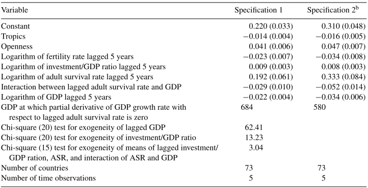
Table 2
Estimated slope coefficients from static random effects models for real per capita GDP growth rates 1965–1990 at 5-year intervals using data from WDIa
Variable Specification 1 Specification 2b
Constant 0.220 (0.033) 0.310 (0.048)
Tropics −0.014 (0.004) −0.016 (0.005)
Openness 0.041 (0.006) 0.047 (0.007)
Logarithm of fertility rate lagged 5 years −0.023 (0.007) −0.034 (0.008) Logarithm of investment/GDP ratio lagged 5 years 0.009 (0.003) 0.008 (0.003) Logarithm of adult survival rate lagged 5 years 0.192 (0.061) 0.333 (0.084) Interaction between lagged adult survival rate and GDP −0.029 (0.010) −0.052 (0.014) Logarithm of GDP lagged 5 years −0.022 (0.004) −0.034 (0.006) GDP at which partial derivative of GDP growth rate with
respect to lagged adult survival rate is zero
684 580
Chi-square (20) test for exogeneity of lagged GDP 62.41 Chi-square (20) test for exogeneity of investment/GDP ratio 13.23 Chi-square (15) test for exogeneity of means of lagged investment/
GDP ration, ASR, and interaction of ASR and GDP
3.04
Number of countries 73 73
Number of time observations 5 5
aAsymptotic standard errors are in parentheses.
bSpecification 1 treats the time varying variables as exogenous; specification 2 treats lagged GDP as a fully endogenous variable.
Because the Chi-square specification test indicated that lagged GDP should be treated as a fully endogenous variable, theR-squared values were computed from reduced form equations regressing lagged GDP on the explanatory variables; the adjustedR-squared for the five time periods were 0.78, 0.80, 0.81, 0.83, and 0.85, respectively. While it is possible to develop a rigorous statistical test for the rank condition underlying the instrumental variable estimation, the adjustedR-squared values suggest that the rank condition is satisfied in this model.
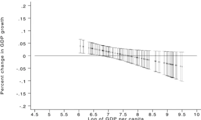
4.2. The net impact of adult survival rates of GDP growth rates
The ASR for a country is likely to be influenced by economic development, access to and quality of medical care, and the public health infrastructure. However, beyond a certain threshold, increases in ASR are difficult to achieve and will increase the proportion of the elderly in the economy. By contrast, for countries at low levels of GDP, one would expect significant effects of ASR on economic growth due to the contribution of labor in prime years. Thus, models for growth rates should allow some forms of non-linearities. Because of the modest number of countries in the data set and because the average life expectancy in the sample was around 60 years, only the interaction between lagged ASR and GDP was found to be statistically significant. For illustrative purposes, we rewrite the net effect of a change in ASR on growth rate as
b1=b2+b3(GDP) (8)
whereb2andb3 are, respectively, the (partial) coefficients of the logarithm of ASR and interaction between logarithms of ASR and GDP in the model (1). The net effectb1can be computed at different levels of GDP and the asymptotic confidence intervals can be approximated from
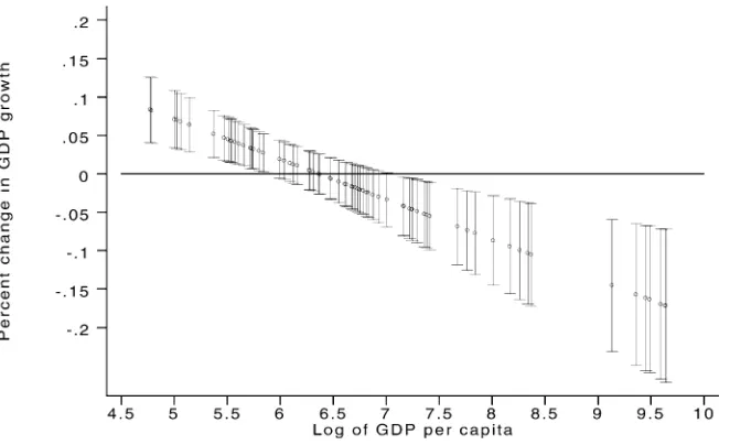
Avar(b1)=Avar(b2)+Avar(b3)(GDP)2+2Acov(b2, b3)(GDP) (9) Thus, we can tabulate the effects of a unit change in ASR on growth rates and the corresponding confidence intervals for the countries at mean GDP levels. The results for
Fig. 2. Net effect and confidence intervals for a percent change in ASR on GDP growth rate using PWT GDP data and assuming GDP is a fully endogenous explanatory variable.
the PWT data are presented in Figs. 1 and 2, where Fig. 2 plots the results for the case where lagged GDP was treated as a fully endogenous variable. The effect was plotted against mean of the logarithm of GDP of countries in the sample period. Corresponding results for the WDI data are in Figs. 3 and 4.
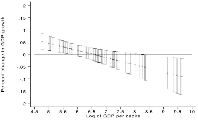
Fig. 4. Net effect and confidence intervals for a percent change in ASR on GDP growth rate using WDI GDP data and assuming GDP is a fully endogenous explanatory variable.
The results from PWT in Fig. 1 showed significant positive effects of ASR on growth rates until the logarithm of the GDP was approximately 6.81 (907 in 1985 international dollars); the corresponding estimate from specification 2 in Fig. 2 was very close. Once these points were crossed, the net effect of ASR approached zero and subsequently assumed negative values. Note, however, that the negative effects of ASR on growth rates were not statistically different from zero in Fig. 1. However, this was not true in Fig. 2, where the net effect was negative and significant for a few countries with high GDP levels.
The results using WDI GDP series in Figs. 3 and 4 were similar for low income countries, except that the threshold where the impact of ASR was zero, was reached earlier. Once the net effect of ASR turned negative, it was statistically significant for certain countries at the high end of the income distribution in Figs. 3 and 4. However, as noted in Section 3.1, this should not be construed as implying harmful effects of ASR on growth rates. Rather, some of the affluent countries, especially in Europe, had achieved high ASR while experiencing slower growth rates in the sample period, due to historical and institutional reasons. As discussed in Section 5, it would be useful to compile additional health indicators providing elaborate information especially in affluent settings.
4.3. Results for the test for reverse causality and parameter stability outside the sample period
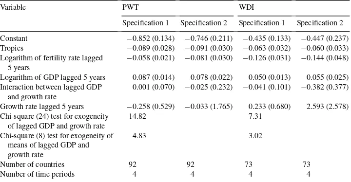
Table 3
Tests for reverse causality based on the slope coefficients from static random effects models for log ASR in the period 1965–1990 at 5-year intervals using the data from PWT and WDIa,b
Variable PWT WDI
Specification 1 Specification 2 Specification 1 Specification 2 Constant −0.852 (0.134) −0.746 (0.211) −0.435 (0.133) −0.447 (0.237) Tropics −0.089 (0.028) −0.091 (0.030) −0.063 (0.032) −0.060 (0.033) Logarithm of fertility rate lagged
5 years
−0.058 (0.021) −0.081 (0.030) −0.126 (0.031) −0.144 (0.048) Logarithm of GDP lagged 5 years 0.087 (0.014) 0.078 (0.022) 0.050 (0.013) 0.055 (0.025) Interaction between lagged GDP
and growth rate
0.001 (0.070) −0.025 (0.232) −0.041 (0.101) −0.382 (0.377) Growth rate lagged 5 years −0.258 (0.529) −0.033 (1.765) 0.233 (0.680) 2.593 (2.578) Chi-square (24) test for exogeneity
Number of countries 92 92 73 73
Number of time periods 4 4 4 4
aSpecifications 1 and 2 treat lagged GDP and growth rate as exogenous and fully endogenous variables, respectively.
bAsymptotic standard errors are in parentheses.
ratios were not significant predictors of ASR; these variables were dropped from the model to reduce multi-collinearity. As expected, lagged GDP level was a significant predictor of ASR. By contrast, lagged GDP growth rate and the interaction between GDP level and growth rate were not statistically significant. The Chi-square statistics for the exogeneity null hypothesis of lagged GDP level and growth rate accepted the null. Overall, the results in Table 3 support the view that lagged GDP growth rates do not influence the current ASR, at least in the short time frame of 5 years. Consequently, the positive associations between ASR and GDP growth rates reported in Tables 1 and 2 are more likely to reflect causality running from ASR to growth rates for low income countries.
5. Conclusion
This paper modeled the proximate determinants of economic growth at 5-year intervals using panel data on GDP series based on purchasing power parities from the PWT and on exchange rate conversions from the WDI. In the conceptual framework of the analysis, the demographic literature relating life expectancy to income (Preston, 1976) was integrated with models commonly specified for economic growth (Barro and Sala-i-Martin, 1995). Appropriate econometric estimators and test procedures were used in the analysis to draw inferences. Although the health of individuals in a country can only be roughly approximated in national averages, the models showed significant effects of ASR on economic growth rates for low income countries. Thus, for example, for the poorest countries, a 1% change in ASR was associated with an approximate 0.05% increase in growth rate. While the magnitude of this coefficient was small, a similar increase of 1% in investment/GDP ratio was associated with a 0.014% increase in growth rate. A novel aspect of the analysis was that we estimated the threshold point beyond which ASR had typically negligible effects on growth rates; confidence intervals for the net impact of ASR highlighted the asymmetries for poor and rich countries (Figs. 1–4). Thus, for example, using the GDP data for 1990 from the PWT, the parameter estimates imply large positive effects of ASR on growth rates for countries in the sample such as Burkina Faso, Burundi and the Central African Republic. The positive effects were also significant for India, Ivory Coast and Nigeria. For highly developed countries such as USA, France and Switzerland, the estimated effect of ASR on growth rates was negative. These empirical findings in part result from the choice of the functional form, explanatory variables available for the analysis, and the standard errors of the estimated parameters.
From a conceptual standpoint, it is important that future research compile more elaborate data on health indicators. Thus, for example, ASR in poor countries reflects the levels of nutrition, smoking prevalence rates, infectious diseases, health infrastructure, and factors such as accidents leading to premature deaths. By contrast, differences in ASR in middle and high income countries may be influenced by genetic factors and by access to and costs of preventive and curative health care. Because investments in skill acquisition in poor countries depend on the ASR, the years for which skilled labor remains productive is likely to be important for explaining economic productivity. Furthermore, it would be useful to augment statistics such as percentages of skilled and unskilled labor compiled for countries (International Labour Organization, 1999) by measures of physical and mental health. For example, productivity loss due to ill health can be estimated from augmenting employment surveys with a health module. Measures of cognitive function in different age cohorts may also be useful for explaining economic performance of countries. Analyses based on elaborate data sets would afford sharper insights into the likely impact of health on economic growth.
Acknowledgements
for their valuable help. This revision has benefited from the comments of a referee and the editor. The views contained in the paper are those of the authors.
References
Ahmad, S., 1992. Regression estimates of per capita GDP based on purchasing power parities. Working Paper #WPS 956, International Economics Department, The World Bank, Washington, DC.
Anderson, T.W., 1971. Statistical Analysis of Time Series. Wiley, New York. Barro, R.J., 1997. Determinants of Economic Growth. MIT Press, Cambridge, MA. Barro, R.J., Sala-i-Martin, X., 1995. Economic Growth. McGraw-Hill, New York.
Barro, R.J., Lee, J.W., 1996. International measures of school years and schooling quality. American Economic Review, Papers and Proceedings 86, 218–223.
Basta, S.S., Soekirman, M.S., Karyadi, D., Scrimshaw, N.S., 1979. Iron deficiency anemia and the productivity of adult males in Indonesia. American Journal of Clinical Nutrition 32, 916–925.
Bhargava, A., 1991a. Identification and panel data models with endogenous regressors. Review of Economic Studies 58, 129–140.
Bhargava, A., 1991b. Estimating short and long run income elasticities of foods and nutrients for rural south India. Journal of the Royal Statistical Society A 154, 174–175.
Bhargava, A., 1997. Nutritional status and the allocation of time in Rwandese households. Journal of Econometrics 77, 277–295.
Bhargava, A., 1998. A dynamic model for the cognitive development of Kenyan schoolchildren. Journal of Educational Psychology 90, 162–166.
Bhargava, A., 2002. Family planning, gender differences and infant mortality: evidence from Uttar Pradesh, India. Journal of Econometrics, in press.
Bhargava, A., 1999. Modeling the effects of nutritional and socioeconomic factors on the growth and morbidity of Kenyan school children. American Journal of Human Biology 11, 317–326.
Bhargava, A., 2000. Stochastic specification and the international GDP series. Discussion Paper, University of Houston.
Bhargava, A., Sargan, J.D., 1983. Estimating dynamic random effects models from panel data covering short time periods. Econometrica 51, 1635–1660.
Bloom, D., Canning, D., 2000. Health and wealth of nations. Science 287, 1207–1209.
Bos, E., 1998. Basic demographic, health and health systems data. Technical Report, The World Bank, Washington, DC.
Boskin, M., Lau, L.J., 1992. Post-war economic growth in the group-of-five countries: a new analysis. Discussion Paper, Stanford University.
Caselli, F., Esquivel, G., Lefort, F., 1996. Reopening the convergence debate: a new look at cross-country growth empirics. Journal of Economic Growth 1, 363–389.
Christensen, L.R., Jorgenson, D.W., Lau, L.J., 1973. Transcendental logarithmic production frontiers. Review of Economics and Statistics 55, 28–45.
Cochrane, W.G., 1965. The planning of observational studies of human populations (with discussion). Journal of the Royal Statistical Society A 128, 234–265.
Collins, S.M., Bosworth, B.P., 1996. Economic growth in East Africa: accumulation versus assimilation. Brookings Papers on Economic Activity 2, 135–203.
Cox, D.R., 1992. Causality: some statistical aspects. Journal of the Royal Statistical Society A 155, 291–302. Fisher, R.A., 1973. Statistical Methods for Research Workers, 14th Edition. Hafner, New York.
Floud, R., Wachter, K., Gregory, A., 1991. Height, Health and History. Cambridge University Press, Cambridge. Fogel, R.W., 1994. Economic growth, population health and physiology: the bearing of long-term processes on
the making of economic policy. American Economic Review 84, 369–395.
Gallup, J.L., Sachs, J.D., 1998. Geography and economic development. Discussion Paper, Center for International Development, Harvard University, Cambridge, MA.
International Institute of Population Sciences, 1995. The national family health survey, Mumbai, India. International Labour Organization, 1999. Key indicators of labour market. International Labour Organization,
Geneva, Switzerland.
Kim, J.I., Lau, L.J., 1994. The sources of economic growth in the East Asian newly industrialized countries. Journal of Japanese and International Economies 8, 235–271.
Murray, C.J.L., Lopez, A., 1996. The Global Burden of Disease. Harvard University Press, Cambridge. Nehru, V., Dhareshwar, A., 1993. A new database on physical capital stock: sources, methodology and results.
Revista de Aanalisis Economico 8, 37–59.
Preston, S.H., 1976. Mortality Patterns in National Populations. Academic Press, New York.
Sala-i-Martin, X., 1996. The classical approach to convergence analysis. Economic Journal 106, 1019–1036. Sargan, J.D., 1958. The estimation of economic relationships using instrumental variables. Econometrica 26,
393–415.
Sargan, J.D., 1964. Wages and prices in the UK: a study in econometric methodology. In: Hart, P., Mills, G., Whitaker, J.K. (Eds.), Econometric Analysis for National Economic Planning. Butterworths, London, pp. 25–54.
Sargan, J.D., 1971. Production functions. In: Layard, P.R.G., Sargan, J.D., Ager, J.D.M.E., Jones, D.J. (Eds.), Qualified Manpower and Economic Performance, Part 5. Allen Lane, London.
Sargan, J.D., 1980. Some tests of dynamic specification for single equations. Econometrica 48, 879–898. Scrimshaw, N.S., 1996. Nutrition and health from womb to tomb. Nutrition Today 31, 55–67.
Scrimshaw, N.S., Taylor, C.E., Gordon, J.E., 1959. Interactions of nutrition and infection. American Journal of Medical Science 237, 367–403.
Spurr, G.B., 1983. Nutritional status and physical work capacity. Yearbook of Physical Anthropology, volume 26, pp. 1–35.
Strauss, J., Thomas, D., 1998. Health, nutrition and economic development. Journal of Economic Literature 36, 766–817.
Stronks, K., van de Mheen, H., van den Bos, J., Makenbach, J.P., 1997. The interrelationship between income, health and employment status. International Journal of Epidemiology 26, 592–599.
Summers, R., Heston, A., 1991. The Penn world table (mark 5): an expanded set of international comparisons, 1950–1988. Quarterly Journal of Economics 6, 327–368.