Statistics authors titles recent submissions

(1)

arXiv:1709.05906v2 [stat.ME] 30 Sep 2017

Bayesian analysis of three parameter singular

Marshall-Olkin bivariate Pareto distribution

Biplab Paul, Arabin Kumar Dey and Debasis Kundu

Department of Mathematics, IIT Guwahati

Department of Mathematics and Statistics, IIT Kanpur

October 3, 2017

Abstract

This paper provides bayesian analysis of singular Marshall-Olkin bivariate Pareto

distribution. We consider three parameter singular Marshall-Olkin bivariate Pareto

distribution. We consider two types of prior - reference prior and gamma prior.

Bayes estimate of the parameters are calculated based on slice cum gibbs sampler

and Lindley approximation. Credible interval is also provided for all methods and all

(2)

(3)

1 Introduction

Bivariate Pareto distribution (BVPA) is used in modelling data related to climate,

network-security etc. A variety of bivariate (multivariate) extensions of the Pareto distribution also

have been considered in the literature. These include the distributions of Sankaran and Kundu

(2014), Yeh (2000), Yeh (2004), Asimit et al. (2010).

In this paper we consider a special type of bivariate Pareto distribution, namely

Marshall-Olkin bivariate Pareto (MOBVPA) whose marginals are type-II univariate Pareto

distribu-tions. We use the notation MOBVPA for singular version of this bivariate Pareto. Finding

efficient estimation technique to estimate the parameters of BVPA was a major challenge

for last few decades. The problem is attempted by some authors in frequentist set up

through EM algorithm [Asimit et al. (2016), Dey and Paul (2017)]. There is no work in

bayesian set up for singular Marshall-Olkin bivariate Pareto distribution. In this paper we

restrict ourselves only up to three parameter MOBVPA.

The bayes estimator can not be obtained in closed form. Therefore we propose to use

two methods. (1) Lindley approximation [Lindley (1980)] (2) Slice cum Gibbs Sampler

[Neal (2003), Casella and George (1992)]. However we can use other Monte Carlo methods

for the same. In this paper we made slight modification in calculation of the Lindley

ap-proximation. We use EM algorithms instead of MLE. We also calculate credible intervals

for the parameters. Bayes estimators exist even when MLEs do not exist. Also Bayesian

estimators may work reasonably well with suitable choice of prior even when MLE’s

per-formance is extremely poor. Therefore working in bayesian set up with such a complicated

distribution has its own advantages. In this paper both informative prior like gamma prior

and non-informative prior like reference prior is used.

(4)

singular Marshall-Olkin bivariate Pareto distribution. Numerical results are discussed in

section 3. In section 4, A data analysis is shown for illustrative purpose. We conclude the

paper in section 5.

2 Bayesian Analysis of singular Marshall-Olkin

bivari-ate Pareto distribution

A random variable X is said to have Pareto of second kind, i.e.

X ∼P a(II)(µ, σ, α) if it has the survival function

¯

FX(x;µ, σ, α) =P(X > x) = (1 +

x−µ

σ )

−α

and the probability density function (pdf)

f(x;µ, σ, α) = α

σ(1 +

x−µ

σ )

−α−1

with x > µ∈ R, σ >0 and α >0.

LetU0, U1andU2are mutually independent random variable whereU0 ∼P A(II)(0,1, α0),

U1 ∼P A(II)(µ1, σ1, α1) andU2 ∼P A(II)(µ2, σ2, α2). We define X1 = min{µ1+σ1U0, U1}

andX2 = min{µ2+σ2U0, U2}, then the joint distribution of (X1, X2) is called the

(5)

distri-bution. The joint survival function of (X1, X2) can be written as;

so it’s pdf that can be written as

(6)

where

The likelihood function corresponding to this pdf is given by,

(7)

Therefore log-likelihood function takes the form,

We assume that α0, α1, and α2 are distributed according to the gamma distribution with

shape parameters ki and scale parameters θi, i.e.,

α0 ∼Γ(k0, θ0)≡Gamma(k0, θ0)

α1 ∼Γ(k1, θ1)≡Gamma(k1, θ1)

α2 ∼Γ(k2, θ2)≡Gamma(k2, θ2) (3)

The probability density function of the Gamma Distribution is given by,

(8)

2.2.2 Reference Prior Assumption

We calculate the expression using Bernardo’s reference Prior [Berger et al. (1992), Bernardo

(1979)] in this context. The following priors are applicable in finding directly the

condi-tional posterior distribution of one parameter given the others and the data. We use

conditional prior of one parameter given the others instead of proposing the unconditional

ones. Since we are planning to use Slice cum Gibbs sampler, we do not need the

expres-sion of full posterior distribution. Writing the joint unconditional prior will lead to a very

complicated expression. We avoid the same and directly write the conditional distribution

of one parameter given the others.

The expressions are as follows :

P0 =π(α0|α1, α2) ∝

In this section we provide the bayes estimates of the unknown parameters namely α0, α1,

(9)

cum Gibbs Sampler method. In this paper we use step-out slice sampling as described by

Neal (2003). We can provide the expression of full posterior when posterior is constructed

based on Gamma prior. The full posterior of (α0, α1, α2) given the data D2 based on the

posterior mean of g, i.e.

(10)

2.4 The Full log- conditional posterior distributions in Gamma

(11)

unconditional ones. Since we are planning to use Slice cum Gibbs sampler, we do not need

the expression of full posterior distribution. Writing the joint unconditional prior will lead

to a very complicated expression. We avoid the same and directly write the conditional

distribution of one parameter given the others. The expressions are as follows :

(12)

2.5 General Lindley Approximation

We use Lindley Approximation (Lindley (1980)) technique to approximate (6) which is

same as approximate evaluation of integral of the form :

R

Let us considerxas a sample of size n taken from a population with probability density function f(x|θ) and X be the corresponding random variable. Let’s denote the likelihood function as l(θ|x) and log-likelihood function as L(θ|x).

We assume thatπ(θ) is a prior distribution of θ and g(θ) is any arbitrary function ofθ.

Under squared error loss function, the bayes estimate of g(θ) is the posterior mean ofg(θ).

Then the Bayes estimate of g(θ) is, After simplification we can write the equation (9) as

(13)

where i, j, k, l= 1,2,3,· · ·, k. Many partial derivatives occur in RHS of the equation (10). Here Lijk is the third order partial derivative with respect to αi, αj, αk, whereas gi is the

first order partial derivative with respect to αi and gij is the second order derivative with

respect to αi and αj. We denote σij as the (i, j)-th element of the inverse of the matrix

{Lij}. All term in right hand side of the equation (10) are calculated at MLE ofθ(= ˆθ,say).

2.6 Lindley Approximation for 3-Parameter singular MOBVPA:

Letα0, α1, α2 be the parameters of corresponding distribution andπ(α0, α1, α2) is the joint

prior distribution of α0, α1 and α2. Then the bayes estimate of any function of α0, α1 and

α2, say g =g(α0, α1, α2) under the squared error loss function is,

ˆ

gB = R

(α0,α1,α2)g(α0, α1, α2)e[L(α0

,α1,α2)+ρ(α0,α1,α2)]_d₍_α

0, α1, α2) R

(α0,α1,α2)e[L(α0,α1,α2)+ρ(α0,α1,α2)]d(α0, α1, α2)

(11)

whereL(α0, α1, α2) is log-likelihood function andρ(α0, α1, α2) is logarithm of joint prior

of α0, α1 and α2 i.e ρ(α0, α1, α2) = logπ(α0, α1, α2). By the Lindley approximation, (??)

can be written as,

ˆ

gB =g( ˆα0,αˆ1,αˆ2) + (g0b0+g1b1+g2b2+b3+b4) +

1

2[A(g0σ00+g1σ01+g2σ02) +B(g0σ10+g1σ11+g2σ12) +C(g0σ20+g1σ21 +g2σ22)]

(14)

(15)

ρ1 = k1_α1−1 −_θ11, ρ2 = k2_α2−1 −_θ21.

L00 =−

n2

( ˆα0+ ˆα1)2

− n1

( ˆα0+ ˆα2)2

− n0

α2 0

L11 =−

n1

( ˆα1)2

− n2

( ˆα0+ ˆα1)2

L22 =−

n1

( ˆα0+ ˆα2)2

L01 =−

n2

( ˆα0+ ˆα1)2

=L10

L02 =−

n1

( ˆα0+ ˆα2)2

=L20

(16)

the values of Lijk for i, j, k = 0,1,2 are given by

Now we can obtain the Bayes estimates of α0, α1 and α2 under squared error loss

(17)

(iii) For α2, chooseg(α0, α1, α2) =α2. So bayes estimates ofα2 can be written as,

ˆ

α2B = ˆα2+b2 +

1

2[Aσ02+Bσ12+Cσ22] (14)

Remark : We replace MLE by its estimates obtained through EM algorithm Dey and Paul

(2017) while calculating the Lindley approximation.

3 Constructing credible Intervals for

θ

We find the credible intervals for parameters as described by Chen and Shao Chen and Shao

(1999). Let assume θ is vector. To obtain credible intervals of first variable θ1i, we order

{θ1i}, as θ1(1) < θ1(2) <· · ·< θ1(M). Then 100(1 - γ)% credible interval of θ1 become

(θ1(j), θ1(j+M−M γ)), f or j = 1,· · · , M γ

Therefore 100(1 -γ)% credible interval for θ1 becomes (θ1(j∗₎, θ_1(j∗_+M₋_{M γ)}), wherej∗ is such that

θ1(j∗_+M₋_{M γ)}−θ_1(j∗₎≤θ_1(j+M₋_{M γ)}−θ_1(j)

for all j = 1,· · · , M γ. Similarly, we can obtain the credible interval for other co-ordinates of θ.

We have scope to construct such intervals when full posterior is not known and tractable.

In this paper we calculate the bayesian confidence interval for both gamma prior and

reference prior. We skip working with full expression of posterior under reference prior as

(18)

4 Numerical Results

The numerical results are obtained by using package R 3.2.3. The codes are run at IIT

Guwahati computers with model : Intel(R) Core(TM) i5-6200U CPU 2.30GHz. The codes

will be available on request to authors.

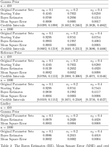
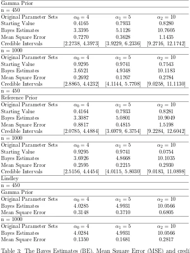
We use the following hyper parameters of prior as gamma : k0 = 2, θ0 = 3, k1 = 4, θ1 =

3, k2 = 3, θ2 = 2. Bayes estimates, mean square errors, credible intervals are calculated for

all the parametersα0,α1 andα2 using both gamma prior and reference prior. Table-6 and

Table-6 show the results obtained by different methods, e.g. Lindley and Slice sampling

etc with different set of priors like Gamma and reference for two different parameter sets.

In slice cum gibbs sampling we take burn in period as 500. Bayes estimates are calculated

based on 2000 and more iterations after burn-in period. We make further investigation on

sample size needed for all the methods to work. We observe that Slice-cum gamma works

even for a sample size like 50 for small parameter values in case of singular MOBVPA. When

original sample is drawn from parameters little bigger, sample size needed to converge the

algorithm becomes more. Slice-cum Gibbs with reference prior as prior requires slightly

more sample size like 250 or more to converge. However Lindley approximation works for

sample size around 150 in almost all cases.

5 Data Analysis

We study the two data sets used in two previous papers Dey and Paul (2017). This data

set is used to model singular Marshall-Olkin bivariate Pareto distribution. We get the

estimates of parameters through EM algorithm for singular Marshall-Olkin bivariate Pareto

distribution as µ1 = 0.0158, µ2 = 0.0012, σ1 = 3.0647, σ2 = 1.9631, α0 = 2.5251, α1 =

(19)

which will model three parameter MOBVPA is not available. Therefore we modify the data

with location and scale transformation. This transformation will affect cardinalities of I0,

I1 and I2 and thereby the value of likelihood function in singular MOBVPA significantly.

Therefore we modified the algorithm by making a suitable approximation of the number

of observations in each of I0, I1 and I2 while calculating the value of likelihood function.

We replace n0, n1 and n2, the cardinality of cells I0, I1 and I2 by ñ0, ñ1 and ñ2 where

˜

ni = (n0 +n1 + n2)_(α0+α1+α2αi ₎ for i = 0,1,2. This approximation can be obtained by

using the distribution of unknown random cardinalities as multinomial distribution with

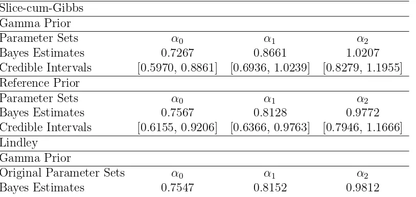
parameter (n0+n1+n2) and _(α0_+α1αi_+α2₎ fori= 0,1,2. Bayes estimates and credible intervals

are calculated and provided in Table-??. Slice-cum-Gibbs

Gamma Prior

Parameter Sets α0 α1 α2

Bayes Estimates 0.7267 0.8661 1.0207

Credible Intervals [0.5970, 0.8861] [0.6936, 1.0239] [0.8279, 1.1955] Reference Prior

Parameter Sets α0 α1 α2

Bayes Estimates 0.7567 0.8128 0.9772

Credible Intervals [0.6155, 0.9206] [0.6366, 0.9763] [0.7946, 1.1666] Lindley

Gamma Prior

Original Parameter Sets α0 α1 α2

Bayes Estimates 0.7547 0.8152 0.9812

(20)

6 Conclusion

Bayes estimates of the parameters of singular bivariate Pareto under square error loss are

obtained both using Lindley and Slice cum Gibbs sampler approach. Both the methods are

working quite well even for moderately large sample size. In case of singular MOBVPA the

algorithms work even for small sample size like 50. Use of informative prior like Gamma

and non-informative prior like reference prior is studied in this context. Posterior using full

reference prior requires more attention. The same study can be made using many other

algorithms like importance sampling, HMC etc. This study can be used to find out bayes

factor between two or more bivariate distributions which can be an appropriate criteria for

discriminating two or more higher dimensional distributions. More work is needed in this

direction. The work is in progress.

References

Asimit, A. V., Furman, E., and Vernic, R. (2010). On a multivariate pareto distribution.

Insurance: Mathematics and Economics, 46(2):308–316.

Asimit, A. V., Furman, E., and Vernic, R. (2016). Statistical inference for a new class of

multivariate pareto distributions. Communications in Statistics-Simulation and Compu-tation, 45(2):456–471.

Berger, J. O., Bernardo, J. M., et al. (1992). On the development of reference priors.

Bayesian statistics, 4(4):35–60.

(21)

Casella, G. and George, E. I. (1992). Explaining the gibbs sampler. The American Statis-tician, 46(3):167–174.

Chen, M.-H. and Shao, Q.-M. (1999). Monte carlo estimation of bayesian credible and hpd

intervals. Journal of Computational and Graphical Statistics, 8(1):69–92.

Dey, A. K. and Paul, B. (2017). Some variations of em algorithms for marshall-olkin

bivariate pareto distribution with location and scale. arXiv preprint arXiv:1707.09974.

Lindley, D. V. (1980). Approximate bayesian methods. Trabajos de estad´ıstica y de inves-tigaci´on operativa, 31(1):223–245.

Neal, R. M. (2003). Slice sampling. Annals of statistics, pages 705–741.

Sankaran, P. and Kundu, D. (2014). A bivariate pareto model. Statistics, 48(2):241–255.

Yeh, H. C. (2000). Two multivariate pareto distributions and their related inferences.

Bulletin of the Institute of Mathematics, Academia Sinica., 28(2):71–86.

Yeh, H.-C. (2004). Some properties and characterizations for generalized multivariate

(22)

Slice-cum-Gibbs Gamma Prior n = 450

Original Parameter Sets α₀ = 0.1 α₁ = 0.2 α₂ = 0.4

Starting Value 0.4165 0.7933 0.8250

Bayes Estimates 0.0768 0.2056 0.4314

Mean Square Error 0.0008 0.0005 0.0017

Credible Intervals [0.0399, 0.1098] [0.1652, 0.2463] [0.3826, 0.4862] n = 1000

Starting Value 0.9295 0.9741 0.0754

Bayes Estimates 0.0903 0.1957 0.4083

Credible Intervals [0.0602, 0.1218] [0.1640, 0.2313] [0.3686, 0.4466] Reference Prior

n = 450

Starting Value 0.4165 0.7933 0.8280

Bayes Estimates 0.0139 0.2652 0.4920

Starting Value 0.9295 0.9741 0.7543

Bayes Estimates 0.0858 0.1982 0.4117

n = 450 Gamma Prior

Bayes Estimates 0.0979 0.2020 0.4028

n = 1000

Bayes Estimates 0.0986 0.2015 0.4018

(23)

Slice-cum-Gibbs Gamma Prior n = 450

Original Parameter Sets α₀= 4 α₁= 5 α₂ = 10

Starting Value 0.4165 0.7933 0.8280

Bayes Estimates 3.3395 5.1126 10.7605

Starting Value 0.9295 0.9741 0.7543

Bayes Estimates 3.6521 4.9348 10.1183

Reference Prior

Starting Value 0.4164 0.7933 0.8281

Bayes Estimates 3.3087 5.0801 10.9049

Starting Value 0.9295 0.9741 0.0754

Bayes Estimates 3.6926 4.8668 10.1035

n = 450 Gamma Prior

Bayes Estimates 4.0285 4.9931 10.0566

n = 1000

Bayes Estimates 4.0284 4.9931 10.0566