Nathan Wiebe
Quantum Architectures and Computing Group, Microsoft Research, Redmond, WA 98052
Ram Shankar Siva Kumar Microsoft, Redmond, WA 98052
(Dated: November 20, 2017)
Security for machine learning has begun to become a serious issue for present day applications. An important question remaining is whether emerging quantum technologies will help or hinder the security of machine learning. Here we discuss a number of ways that quantum information can be used to help make quantum classifiers more secure or private. In particular, we demonstrate a form of robust principal component analysis that, under some circumstances, can provide an exponential speedup relative to robust methods used at present. To demonstrate this approach we introduce a linear combinations of unitaries Hamiltonian simulation method that we show functions when given an imprecise Hamiltonian oracle, which may be of independent interest. We also introduce a new quantum approach for bagging and boosting that can use quantum superposition over the classifiers or splits of the training set to aggragate over many more models than would be possible classically. Finally, we provide a private form ofk–means clustering that can be used to prevent an all powerful adversary from learning more than a small fraction of a bit from any user. These examples show the role that quantum technologies can play in the security of ML and vice versa. This illustrates that quantum computing can provide useful advantages to machine learning apart from speedups.
I. INTRODUCTION
There is a huge uptick in the use of machine learning for mission critical industrial applications from self driving cars [1] to detecting malignant tumors [2] to detecting fraudulent credit card transactions [3]: machine learning is crucial in decision making. However, classical Machine learning algorithms such as Principal component analysis (used heavily in anomaly detection scenarios), clustering (used in unsupervised learning), support vector machines (used in classification scenarios), as commonly implemented, are extremely vulnerable to changes to the input data, features and the final model parameters/hyper-parameters that have been learned. Essentially, an attacker can exploit any of the above vulnerabilities and subvert ML algorithms. As a result, an attacker has a variety of goals that can be achieved: increasing the false negative rate and thus become undetected (for instance, in the case of spam, junk emails are classified as normal) [4] or by increasing the false positive rate (for instance, in the case of intrusion detection systems, attacks get drowned in sea of noise which causes the system to shift the baseline activity) [5,6,6,7], steal the underlying model itself exploiting membership queries [8] and even recover the underlying training data breaching privacy contracts [8].
In machine learning literature, this study is referred to as adversarial machine learning and has largely been applied to security sensitive areas such as intrusion detection [9,10] and spam filtering [4]. To combat the problem of adversarial machine learning, solutions have been studied from different vantage points: from a statistical stand point, adversaries are treated as noise and thus the models are hardened using robust statistics to overcome the malicious outliers [11]. Adversarial training is a promising trend in this space, is wherein defenders train the system with adversarial examples from the start so that the model is acclimatized to such threats. From a security standpoint, there has been substantial work surrounding threat modeling machine learning systems [12,13] and frameworks for anticipating different kinds of attacks [14].
Quantum computing has experienced a similar surge of interest of late and this had led to a synergistic relationship wherein quantum computers have been found to have profound implications for machine learning [15–27] and machine learning has been shown to be invaluable for characterizing, controlling and error correcting such quantum comput-ers [28–30]. However, as of late the question of what quantum computers can do to protect machine learning from adversaries is relatively underdeveloped. This is perhaps surprising given the impact that applications of quantum computing to security have a long history.
The typical nexus of quantum computing and security is studied from the light of quantum cryptography and its ramifications in key exchange and management. This paper takes a different tack. We explores this intersection by asking questions the use of quantum subroutines to analyze patterns in data, and explores the question and security assurance - specifically, asking the question Are quantum machine learning systems secure?
Our aim is to address this question by investigating the role that quantum computers may have in protecting machine learning models from attackers. In particular, we introduce a robust form of quantum principal component analysis that provides exponential speedups while making the learning protocol much less sensitive to noise introduced
by an adversary into the training set. We then discuss bagging and boosting, which are popular methods for making models harder to extract by adversaries and also serve to make better classifiers by combining the predictions of weak classifiers. Finally, we discuss how to use ideas originally introduced to secure quantum money to boost the privacy ofk-means by obfuscating the private data of participants from even an allpowerful adversary. From this we conclude that quantum methods can be used to have an impact on security and that while we have shown defences against some classes of attacks, more work is needed before we can claim to have a fully developed understanding of the breadth and width of adversarial quantum machine learning.
II. ADVERSARIAL QUANTUM MACHINE LEARNING
As machine learning becomes more ubiquitous in applications so too do attacks on the learning algorithms that they are based on. The key assumption usually made in machine learning is that the training data is independent of the model and the training process. For tasks such as classification of images from imagenet such assumptions are reasonable because the user has complete control of the data. For other applications, such as developing spam filters or intrusion detection this may not be reasonable because in such cases training data is provided in real time to the classifier and the agents that provide the information are likely to be aware of the fact that their actions are being used to inform a model.
Perhaps one of the most notable examples of this is the Tay chat bot incident. Tay was a chat bot designed to learn from users that it could freely interact with in a public chat room. Since the bot was programmed to learn from human interactions it could be subjected to what is known as a wolf pack attack, wherein a group of users in the chat room collaborated to purposefully change Tay’s speech patterns to become increasingly offensive. After 16 hours the bot was pulled from the chat room. This incident underscores the need to build models that can learn while at the same time resist malfeasant interactions on the part of a small fraction of users of a system.
A major aim of adversarial machine learning is to characterize and address such problems by making classifiers more robust to such attacks or by giving better tools for identifying when such an attack is taking place. There are several broad classes of attacks that can be considered, but perhaps the two most significant in the taxonomy in attacks against classifiers are exploratory attacks and causative attacks. Exploratory attacks are not designed to explicitly impact the classifier but instead are intended to give an adversary information about the classifier. Such attacks work by the adversary feeding test examples to the classifier and then inferring information about it from the classes (or meta data) returned. The simplest such attack is known as an evasion attack, which aims to find test vectors that when fed into a classifier get misclassified in a way that benefits the adversary (such as spam being misclassified as ordinary email). More sophisticated exploratory attacks may even try identify to the model used to assign the class labels or in extreme cases may even try identify the training set for the classifier. Such attacks can be deployed as a precursor to causitive attacks or can simply be used to violate privacy assumptions that the users that supplied data to train the classifier may have had.
Causitive attacks are more akin to the Tay example. The goal of such attacks is to change the model by providing it with training examples. Again there is a broad taxonomy of causitive attacks but one of the most ubiquitous attacks is the poisoning attack. A poisoning attack seeks to control a classifier by introducing malicious training data into the training set so that the adversary can force an incorrect classification for a subset of test vectors. One particularly pernicious type of attack is the boiling frog attack, wherein the amount of malicious data introduced in the training set is slowly increased over time. This makes it much harder to identify whether the model has been compromised by users because the impact of the attack, although substantial, is hard to notice on the timescale of days.
While a laundry list of attacks are known against machine learning systems the defences that have been developed thus far are somewhat limited. A commonly used tactic is to replace classifiers with robust versions of the same classifier. For example, considerk–means classification. Such classifiers are not necessarily robust because the intra-cluster variance is used to decide the quality of a intra-clustering. This means that an adversary can provide a small number of training vectors with large norm that can radically impact the cluster assignment. On the other hand, if robust statistics such as the median, are used then the impact that the poisoned data can have on the cluster centroids is minimal. Similarly, bagging can also be used to address these problems by replacing a singular classifier that is trained on the entire training set with an ensemble of classifiers that are trained on subsets the training set. By aggragating over the class labels returned by this process we can similarly limit the impact of an adversary that controls a small fraction of the data set.
isometries,UQRAM|ji|0i=|ji|[vj]iwhere [vj] is a qubit string used to encode thejth training vector. Similarly such an oracle can be used to implement a second type of oracle which outputs the vector as a quantum state vector (we address the issue of non-unit norm training examples below): U|ji|0i =|ji|vji. Alternatively, one can consider a density matrix query for use in an LMR algorithm for density matrix exponentiation [31,32] wherein a query to the training data takes the formB|0i 7→ρwhere ρis a density operator that is equivalent the distribution over training vectors. For example, if we had a uniform distribution over training vectors in a training set of N training vectors thenρ=PNj=1|vjihvj|/(TrPNj=1|vjihvj|).
With such quantum access models defined we can now consider what it means to perform a quantum poisoning attack. A poisoning attack involves an adversary purposefully altering a portion of the training data in the classical case so in the quantum case it is natural to define a poisoning attack similarly. In this spirit, a quantum poisoning attack takes some fraction of the training vectors,η, and replaces them with training vectors of their choosing. That is to say, if without loss of generality an adversary replaces the firstηN training vectors in the data set then the new oracle that the algorithm is provided is of the form
UQRAM|ji|0i=
(
|ji|[vj]i , ifj > ηN
|ji|[φj]i , otherwise, (1)
where|[φj]iis a bit string of the adversary’s choice. Such attacks are reasonable if a QRAM is stored on an untrusted machine that the adversary has partial access to, or alternatively if the data provided to the QRAM is partially under the adversary’s control. The case where the queries provide training vectors, rather than qubit vectors, is exactly the same. The case of a poisoning attack on density matrix input is much more subtle, however in such a case we define the poisoning attack to take the formB|0i=ρ′ : |Tr(ρ−ρ′)| ≤η, however other definitions are possible.
Such an example is a quantum causitive attack since it seeks to cause a change in the quantum classifier. An example of a quantum exploratory attack could be an attack that tries to identify the training data or the model used in the classification process. For example, consider a quantum nearest neighbor classifier. Such classifiers search through a large database of training examples in order to find the closest training example to a test vector that is input. By repeatedly querying the classifier using quantum training examples adversarially chosen it is possible to find the decision boundaries between the classes and from this even the raw training data can, to some extent, be extracted. Alternatively one could consider cases where an adversary has access to the network on which a quantum learning protocol is being carried out and seeks to learn compromising information about data that is being provided for the training process, which may be anonymized at a later stage in the algorithm.
Quantum can help, to some extent, both of these issues. Poisoning attacks can be addressed by building robust classifiers. That is, classifiers that are insensitive to changes in individual vectors. We show that quantum technologies can help with this by illustrating how quantum principal component analysis and quantum bootstrap aggragation can be used to make the decisions more robust to poisoning attacks by proposing new variants of these algorithms that are ammenable to fast quantum algorithms for medians to be inserted in the place of the expectation values typically used in such cases. We also illustrate how ideas from quantum communication can be used to thwart exploratory attacks by proposing a private version of k–means clustering that allows the protocol to be performed without (substantially) compromising the private data of any participants and also without requiring that the individual running the experiment be authenticated.
III. ROBUST QUANTUM PCA
The idea behind principal component analysis is simple. Imagine you have a training set composed of a large number of vectors that live in a high dimensional space. However, often even high dimensional data can have an effective low-dimensional approximation. Finding such representations in general is a fine art, but quantum principal component analysis provides a prescriptive way of doing this. The idea of principal component analysis is to examine the eigenvectors of the covariance matrix for the data set. These eigenvectors are the principal components, which give the directions of greatest and least variance, and their eigenvalues give the magnitude of the variation. By transforming the feature space to this eigenbasis and then projecting out the components with small eigenvalue one can reduce the dimensionality of the feature space.
overlap with the eigenvectors with large eigenvalue, and if it is not then it should have high overlap with the small eigenvectors.
While this technique can be used in practice it can have a fatal flaw. The flaw is that an adversary can inject spikes of usage in directions that align with particular principal components of the classifier. This allows them to increase the variance of the traffic along principal components that can be used to detect their subsequent nefarious actions. To see this, let us restrict our attention to poisoning attacks wherein an adversary controls some constant fraction of the training vectors.
Robust statistics can be used to help mitigate such attacks. The way that it can be used to help make PCA secure is by replacing the mean with a statistic like the median. Because the median is insensitive to rare but intense events, an adversary needs to control much more of the traffic flowing through the system in order to fool a classifier built to detect them. For this reason, switching to robust PCA is a widely used tactic to making principal component analysis more secure. To formalize this, let us define what the robust PCA matrix is first.
Definition 1. Letxj :j= 1 :N be a set of real vectors and letek:k= 1, . . . , Nvbe basis vectors in the computational basis then we define Mk,ℓ:= median([eT
kxj−median(eTkxj)][eTℓxj−median(eTℓxj)]). This is very similar to the PCA matrix when we can express as mean([eT
kxj−mean(eTkxj)][eTℓxj−mean(eTℓxj)]). Because of the similarity that it has with the PCA matrix, switching from a standard PCA algorithm to a robust PCA algorithm in classical classifiers is a straight forward substitution.
In quantum algorithms, building such robustness into the classifier is anything but easy. The challenge we face in doing so is that the standard approach to this uses the fact that quantum mechanical state operators can be viewed as a covariance matrix for a data set [31,32]. By using this similarity in conjunction with the quantum phase estimation algorithm the method provides an expedient way to project onto the eigenvectors of the density operator and in turn the principal components. However, the robust PCA matrix given in 1 does not have such a natural quantum analogue. Moreover, the fact that quantum mechanics is inherently linear makes it more challenging to apply an operation like the median which is not a linear function of its inputs. This means that if we want to use quantum PCA in an environment where an adversary controls a part of the data set, we will need to rethink our approach to quantum principal component analysis.
The challenges faced by directly applying density matrix exponentiation also suggests that we should consider quantum PCA within a different cost model than that usually used in quantum principal component analysis. We wish to examine whether data obtained from a given source, which we model as a black box oracle, is typical of a well understood training set or not. We are not interested in the principal components of the vector, but rather are interested in its projection onto the low variance subspace of the training data. We also assume that the training vectors are accessed in an oracular fashion and that nothing apriori is known about them.
Definition 2. LetU be a self-adjoint unitary operator acting on a finite dimensional Hilbert space such thatU|ji|0i= |ji|vjiwherevj is thejth training vector.
Lemma 3. Let xj ∈CN for integer j in [1, Nv] obey kxjk ≤R ∈R. There exists a set of unit vectors in a Hilbert
space of dimensionN(2Nv+ 1)such that for any|xji,|x†kiwithin this sethx†j|xki=hxj, xki/R2.
Proof. The proof is constructive. Let us assume thatR >0. First let us define for anyxj,
|xj/kxjki:=xj/kxjk. (2) We then encode
xj7→ |xji:=|xj/kxjki kxjk R |0i+
r
1−kxjk 2
R2 |ji
!
.
x†j7→ |x†ji:=|x†j/kxjki k xjk R |0i+
r
1−kxjR2k2|j+Nvi
!
. (3)
IfR= 0 then
xj7→ |0i|ji,
For the above reason, we can assume without loss of generality that all training vectors are unit vectors. Also for simplicity we will assume thatvj ∈R, but the complex case follows similarly and only differs in that both the real
and imaginary components of the inner products need to be computed.
Threat Model 1. Assume that the user is provided an oracle, U, that allows the user to access real-valued vectors of dimension as quantum states yielded by an oracle of the form inLemma 3. This oracle could represent an efficient quantum subroutine or it could represent a QRAM. The adversary is assumed to have control with probabilityα <1/2
the vector|xjiyielded by the algorithm for a given coherent query subject to the constraint thatkxjk ≤R. The aim of the adversary is to affect, through these poisoned samples, the principal components yielded from the data set yielded byU.
Within this threat model, the maximum impact that the adversary could have on any of the expectation values that form the principal component matrix O(αR). Thus any given component of the principal component matrix can be controlled by the adversary provided that the data expectationα≫µ/Rwhere µis an upper bound on the componentwise means of the data set. In other words, ifαis sufficiently large and the maximum vector length allowed within the algorithm is also large then the PCA matrix can be compromised. This vulnerability comes from the fact that the mean can be dominated by inserting a small number of vectors with large norm.
Switching to the median can dramatically help with this problem as shown in the following lemma, whose proof is trivial but we present for completeness.
Lemma 4. Let P(x) be a probability distribution on R with invertable cummulative distribution function CDF.
Further, let CDF−1 be its inverse cummulative distribution function and let CDF−1 be Lipshitz continuous with Lipshitz constant L on [0,1]. Assume that an adversary replaces P(x) with a distribution Q(x) that is within total variational distanceα <1/2from P(x). Under these assumptions|median(P(x))−median(Q(x))| ≤αL.
Proof. LetRy0
−∞P(x)dx= 1/2 and
Ry0
−∞Q(x)dx= 1/2. We then have from the triangle inequality that
Z y1
−∞
Q(x)dx≤
Z y1
−∞
P(x)dx+
Z ∞
−∞|
P(x)−Q(x)|dx= CDF(y1) +α. (5)
Thus we have that 12−α≤CDF(y1). The inverse cummulative distribution function is a monotonically increasing function on [0,1] which implies along with our assumption of Lipshitz continuity with constantL
y0−Lα= CDF−1
1 2
−Lα≤CDF−1
1 2−α
≤CDF−1(CDF(y1)) =y1. (6)
Using the exact same argument but applying the reverse triangle inequality in the place of the triangle inequality givesy1≤y0+αLwhich completes the proof.
Thus under reasonable continuity assumptions on the unperturbed probability distributionLemma 4 shows that the maximum impact that an adversary can have on the median of a distribution is negligible. In contrast, the mean does not enjoy such stability and as such using robust statistics like the median can help limit the impact of adversarially placed training vectors within a QRAM or alternatively make the classes less sensitive to outliers that might ordinarily be present within the training data.
Theorem 5. Let the minimum eigenvalue gap of d–sparse Hermitian matrix M within the support of the input state beλ, let each training vectorxj be a unit vector provided by the oracle defined inLemma 3 and assume that the underlying data distribution for the components of the training data has a continuous inverse cummulative distribution with function with constant Lipshitz constantL >0. We have that
1. The number of queries needed to the oracle given in Lemma 3 needed to sample from a distribution P over
O(λ)–approximate eigenvalues of M such that for all training vectors x |P(E′
n)− |hx|Eni|2| ≤ Λ ≤ 1 is in O([d4/Λ3λ3] log2(d2/(λΛ))).
2. Assuming an adversary replaces the data distribution used for the PCA task by one within variational distanceα
from the original such thatαL≤1andα <1/2. IfM′ be is the poisoned robust PCA matrix thenkM−M′k2≤ 5αL(d+ 2).
problems with the algorithm. Furthermore, we need to show that the errors in simulation do not have a major impact on the output probability distributions of the samples drawn from the eigenvalues/ vectors of the matrix. We do this using an argument based on perturbation theory under the assumption that all relevant eigenvalues have multiplicity 1. For these reasons, we encourage the interested reader to look at the appendix for all technical details regarding the proof.
From Theorem 5 we see that the query complexity required to sample from the eigenvectors of the robust PCA matrix is exponentially lower in some cases than what would be expected from classical methods. While this opens up the possibility of profound quantum advantages for robust principal component analysis, a number of caveats exist that limit the applicability of this method:
1. The cost of preparing the relevant input data|xiwill often be exponential unless|xitakes a special form. 2. The proofs we provide here require that the gaps in the relevant portion of the eigenvalue spectrum are large
in order to ensure that the perturbations in the eigenvalues of the matrix do not sufficiently large as to distort the support of the input test vector.
3. The matrixMmust be polynomially sparse.
4. The desired precision for the eigenvalues of the robust PCA matrix is inverse polynomial in the problem size. 5. The eigenvalue gaps are polynomially large in the problem size.
These assumptions preclude it from providing exponential advantages in many cases, however, it does not preclude exponential advantages in quantum settings where the input is given by an efficient quantum procedure. Some of these caveats can be relaxed by using alternative simulation methods or exploiting stronger promises about the structure ofM. We leave a detailed discussion of this for future work. The final two assumptions are in practice may be the strongest restrictions for our method, or at least the analysis we provide for the method, because the complexity diverges rapidly with both quantities. It is our hope that subsequent work will improve upon this, perhaps by using more advanced methods based on LCU techniques to eschew the use of amplitude estimation as an intermediate step. Looking at the problem from a broader perspective, we have shown that quantum PCA can be applied to defend againstThreat Model 1. Specifically, we have resilience to . in a manner that helps defend against attacks on the training corpus either directly which allows the resulting classifiers to be made robust to adversaries who control a small fraction of the training data. This shows that ideas from adversarial quantum machine learning can be imported into quantum classifiers. In contrast, before this work it was not clear how to do this because existing quantum PCA methods cannot be easily adapted from using a mean to a median. Additionally, this robustness also can be valuable in non-adversarial settigns becuase it makes estimates yielded by PCA less sensitive to outliers which may not necessarily be added by an adversary. We will see this theme repeated in the following section where we discuss how to perform quantum bagging and boosting.
IV. BOOTSTRAP AGGRAGATION AND BOOSTING
Bootstrap aggragation, otherwise known as bagging for short, is another approach that is commonly used to increase the security of machine learning as well as improve the quality of the decision boundaries of the classifier. The idea behind bagging is to replace a single classifier with an ensemble of classifiers. This ensemble of classifiers is constructed by randomly choosing portions of the data set to feed to each classifier. A common way of doing this is bootstrap aggragation, wherein the training vectors are chosen randomly with replacement from the original training set. Since each vector is chosen with replacement, with high probability each training set will exclude a constant fraction of the training examples. This can make the resultant classifiers more robust to outliers and also make it more challenging for an adversary to steal the model.
We can abstract this process by instead looking at an ensemble of classifiers that are trained using some quantum subroutine. These classifiers may be trained with legitimate data or instead may be trained using data from an adversary. We can envision a classifier, in the worst case, as being compromised if it receives the adversary’s training set. As such for our purposes we will mainly look at bagging through the lens of boosting, which uses an ensemble of different classifiers to assign a class to a test vector each of which may be trained using the same or different data sets. Quantum boosting has already been discussed in [25], however, our approach to boosting differs considerably from this treatment.
The type of threat that we wish to address with our quantum boosting protocol is given below.
Separating hyperplan e Test
vect or
Separ ating
hype rplan
e +1 eigenve
ctors
-1 eige nvectors
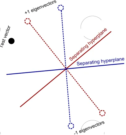
FIG. 1: Eigenspaces for two possible linear classifiers for linearly separated unit vectors. Each trained model provides a different separating hyperplane and eigenvectors. Bagging aggragates over the projections of the test vector onto these eigenvectors and outputs a class based on that aggragation.
0≤α <1of all classifiersCj that the oracle uses to classify data and wishes to affect the classes reported by the user of the boosted quantum classifier that implementsC. The adversary is assumed to have no computational restrictions and complete knowledge of the classifiers / training data used in the boosting protocol.
While the concept of a classifier has a clear meaning in classical computing, if we wish to apply the same ideas to quantum classifiers we run into certain challenges. The first such challenge lies with the encoding of the training vectors. In classical machine learning training vectors are typically bit vectors. For example, a binary classifier can then be thought of as a map from the space of test vectors to {−1,1} corresponding to the two classes. This is if C were a classifier then Cv=±v for all vectorsv depending on the membership of the vector. Thus every training vector can be viewed as an eigenvector with eigenvalue±1. This is illustrated for unit vectors inFigure 1.
Now imagine we instead that our test vector is a quantum state|ψiin C2. Unlike the classical setting, it may be physically impossible for the classifier to know precisely what |ψi is because measurement inherently damages the state. This makes the classification task fundamentally different than it is in classical settings where the test vector is known in its entirety. Since such vectors live in a two-dimensional vector space and they comprise an infinite set, not all |ψican be eigenvectors of the classifierC. However, if we let C be a classifier that has eigenvalue±1 we can always express |ψi=a|φ+i+
p
1− |a|2|φ−i, whereC|φ±i=±|φ±i. Thus we can still classify in the same manner, but now we have to measure the state repeatedly to determine whether|ψihas more projection onto the positive or negative eigenspace of the classifier. This notion of classification is a generalization of the classical idea and highlights the importance of thinking about the eigenspaces of a classifier within a quantum framework.
Our approach to boosting and bagging embraces this idea. The idea is to combine an ensemble of classifiers to form a weighted sum of classifiersC=PjbjCj wherebj>0 and
P
jbj= 1. Let |φibe a simultaneous +1 eigenvector of eachCj, ieCj|φi=|φi
C|φi=X j
bjCj|φi=|φi. (7)
The same obviously holds for any |φi that is a negative eigenvector of each Cj. That is any vector that is in the simultaneous positive or negative eigenspace of each classifier will be deterministically classified byC.
from straight forwardly measuring the expectation of each of the constituentCj to obtain a classification for|ψi. It also prevents us from using quantum state tomography to learn|ψiand then applying a classifier on it. We provide a formal definition of this form of quantum boosting or bagging below.
Definition 6. Two-class quantum boosting or bagging is defined to be a process by which an unknown test vector is classified by projecting it onto the eigenspace of C =PjbjCj and assigning the class to be +1 if the probability of projecting onto the positive eigenspace is greater than1/2 and−1 otherwise. Here eachCj is unitary with eigenvalue
±1,Pjbj= 1,bj≥0, and at least twobj that correspond to distinctCj are positive.
We realize such a classifier via phase estimation. But before discussing this, we need to abstract the input to the problem for generality. We do this by assuming that each classifier,Cj, being included is specified only by a weight vectorwj. If the individual classifiers were neural networks then the weights could correspond to edge and bias weights for the different neural networks that we would find by training on different subsets of the data. Alternatively, if we were forming a committee of neural networks of different structures then we simply envision taking the register used to store wj to be of the form [tag, wj] where the tag tells the system which classifier to use. This allows the same data structure to be used for arbitrary classifiers.
One might wonder why we choose to assign the class based on the mean class output by C rather than the class associated with the mean of C. In other words, we could have defined our quantum analogue of boosting such that the class is given by the expectation value of C in the test state, sign(hψ|C|ψi). In such a case, we would have no guarantee that the quantum classifier would be protected against the adversary. The reason for this is that the mean that is computed is not robust. For example, assume that the ensemble consists ofN classifiers such that for eachCj, |hψ|Cj|ψi| ≤1/(2N) and assume the weights are uniform (if they are not uniform then the adversary can choose to replace the most significant classifier and have an even greater effect). Then if an adversary controls a single classifier example and knows the test example then they could replaceC1such that|hψ|C1|ψi|= 1. The assigned class is then
sign
hψ|C1|ψi N −
1 2N
<sign
hψ|C1|ψi N +
N
X
j=2
hψ|Cj|ψi N
<sign
hψ|C1|ψi N +
1 2N
. (8)
In such an example, even a single compromised classifier can impact the class returned because by pickinghψ|C1|ψi= ±1 the adversary has complete control over the class returned. In contrast, we show that compromising a single quantum classifier does not have a substantial impact on the class if our proposal is used assuming the eigenvalue gap between positive and negative eigenvalues ofC is sufficiently large in the absence of an adversary.
We formalize these ideas in a quantum setting by introducing quantum blackboxes,T,BandC. The first takes an index and outputs the corresponding weight vector. The second prepares the weights for the different classifiers in the ensemble C. The final blackbox applies, programmed via the weight vector, the classifier on the data vector in question. We formally define these black boxes below.
Definition 7. Let C be a unitary operator such that if |wi ∈ C2nw represents the weights that specify the classifier
C|wi|ψi=|wiC(w)|ψifor any state |ψi. Let T be a unitary operator that, up to local isometries performs T |ji|0i= |ji|wji, which is to say that it generates the weights for classifierj (potentially via training on a subset of the data). Finally, define unitaryB:B|0i=Pjpbj|ji for non-negativebj that sum to1.
In order to apply phase estimation onC, for a fixed and unknown input vector,|ψi, we need to be able to simulate e−iCt. Fortunately, because each Cj has eigenvalue±1 it is easy to see thatC2
j = 1 and hence is Hermitian. Thus C is a Hamiltonian. We can therefore apply Hamiltonian simulation ideas to implement this operator and formally demonstrate this in the following lemma.
Lemma 8. Let C =PMj=1bjCj where eachCj is Hermitian and unitary and has a corresponding weight vector wj
for bj ≥ 0 ∀ j and Pjbj = 1. Then for every ǫ > 0 and t ≥ 0 there exists a protocol for implementing a non-unitary operator,W, such that for all|ψi ke−iCt|ψi −W|ψik ≤ǫusing a number of queries toC,B andT that is in O(tlog(t/ǫ)/log log(t/ǫ)).
Proof. The proof follows from the truncated Taylor series simulation algorithm. By definition we have that B|0i=
P
j
p
Next, by assumption we have thatPjbj = 1 and thereforeT =t. Thus the number of queries to select(V) and B in the algorithm is inO(tlog(t/ǫ)/log log(t/ǫ)). The result then follows after noting that a single call to select(V) requiresO(1) calls toV andC.
Note that in general purpose simulation algorithms, the application of select(V) will require a complex series of controls to execute; whereas here the classifier is made programmable via theT oracle and so the procedure does not explicitly depend on the number of terms in C (although in practice it will often depend on it through the cost of implementingT as a circuit). For this reason the query complexity cited above can be deceptive if used as a surrogate for the time-complexity in a given computational model.
With the result ofLemma 8 we can now proceed to finding the cost of performing two-class bagging or boosting where the eigenvalue ofC is used to perform the classification. The main claim is given below.
Theorem 9. Under the assumptions of Lemma 8, the number of queries needed to C, B and T to project
|ψi onto an eigenvector of C with probability at least 1 − δ and estimate the eigenvalue within error ǫ is in
O((δǫ1) log(1/ǫ)/log log(1/ǫ)).
Proof. Since kCk ≤1, it follows that we can apply phase estimation on the e−iC in order to project the unknown state|ψionto an eigenvector. The number of applications ofe−iC needed to achieve this within accuracyǫand error δis O(1/δǫ) using coherent phase estimation [20]. Therefore, after takingt= 1 and using the result ofLemma 8 to simulatee−iC that the overall query complexity for the simulation is inO((1
δǫ) log(1/ǫ)/log log(1/ǫ)).
Finally, there is the question of how large on an impact an adversary can have on the eigenvalues and eigenvectors of the classifier. This answer can be found using perturbation theory to estimate the derivatives of the eigenvalues and eigenvectors of the classifier C as a function of the maximum fraction of the classifiers that the adversary has compromised. This leads to the following result.
Corollary 10. Assume thatC is a classifier defined as per Definition 6that is described by a Hermitian matrix that the absolute value of each eigenvalue is bounded below by γ/2 and that one wishes to perform a classification of a data set based on the mean sign of the eigenvectors in the suport of a test vector. Given that an adversary controls a fraction of the classifiers equal toα < γ/4, the adversary cannot affect the classes output by this protocol in the limit whereǫ→0andδ→0.
Proof. If an adversary controls a fraction of data equal toαthen we can view the perturbed classifier as
C′= (1−Xα)N
j=1
bjCj+ N
X
j=(1−α)N+1
bjCj′ =C+ N
X
j=1
δj>(1−α)Nbj(Cj′−Cj). (9)
This means that we can viewC′as a perturbation of the original matrix by a small amount. In particular, this implies that because eachCj is Hermitian and unitary
kC′−Ck ≤αmax j kC
′
j−Cjk ≤2α. (10)
Using perturbation theory, (see Eq. (A32) in the appendix), we show that the maximum shift in any eigenvalue due to this perturbation is at most 2α. By which we mean that if Ej is the jth eigenvalue of C and C′(σ) = C+σPNj=1δj>(1−α)Nbj(Cj′ −Cj) then the corresponding eigenvalueEj(σ) obeys|Ej(σ)−Ej| ≤2σα+O(σ2). By integrating this we find thatEj(1) (informally the eigenvalue ofC′ corresponding to thejth eigenvalue ofC) we find that|Ej(1)−Ej|=|E′
j−Ej| ≤2α.
Given that Ej ≥γ/2 the above argument shows that sign(Ej) = sign(E′
j) if 2α < γ/2. Thus if the value ofαis sufficiently small then none of the eigenvectors returned will have the incorrect sign. This implies that if we neglect errors in the estimation of eigenvalues ofC then the adversary can only impact the class output byC if they control a fraction greater thanγ/4. In the limit asδ→0 andǫ→0 these errors become negligible and the result follows.
From this we see that adversaries acting in accordance with Threat Model 2 can be thwarted using boosting or bagging that have control over a small fraction of the quantum classifiers used in a boosting protocol. This illustrates that by generalizing the concept of boosting to a quantum setting we can not only make our classifiers better but also make them more resilient to adversaries who control a small fraction of the classifiers provided. This result, combined with our previous discussion of robust quantum PCA, shows that quantum techniques can be used to defend quantum classifiers against causative attacks by quantum adversaries.
V. QUANTUM ENHANCED PRIVACY FOR CLUSTERING
Since privacy is one of the major applications of quantum technologies, it should come as no surprise that quantum computing can help boost privacy in machine learning as well. As a toy example, we will first discuss how quantum computing can be used to allow k–means clustering to be performed without leaking substantial information about any of the training vectors.
Thek–means clustering algorithm is perhaps the most ubiquitous algorithm used to cluster data. While there are several variants of the algorithm, the most common variant attmepts to break up a data set intokclusters such that the sum of the intra-cluster variances is minimized. In particular, letf : (xj,{µ})7→(1, . . . , k) gives the index of the set of centroids {µ} ={µ1, . . . , µk} and xj are the vectors in the data set. Thek–means clustering algorithm then seeks to minimizePj|xj−µf(xj,{µ})|22. Formally, this problem isNP–hard which means that no efficient clustering algorithm (quantum or classical) is likely to exist. However, most clustering problems are not hard examples, which means that clustering generically is typically not prohibitively challenging.
Thek–means algorithm for clustering is simple. First begin by assigning theµp to data points sampled at random. Then for eachxj find theµp that is closest to it, and assign that vector to thepth cluster. Next setµ1, . . . , µk to be the cluster centroids of each of thekclusters and repeat the previous steps until the cluster centroids converge.
A challenge in applying this algorithm to cases, such as clustering medical data, is that the individual performing the algorithm typically needs to have access to the users information. For sensitive data such as this, it is difficult to apply such methods to understand structure in medical data sets that are not already anonymized. Quantum mechanics can be used to address this.
Imagine a scenario where an experimenter wishes to collaboratively cluster a private data set. The experimenter is comfortable broadcasting information about the model to theNowners of the data, but the users are not comfortable leaking more thanmbits of information about their private data in the process of clustering the data. Our approach, which is related to quantum voting strategies [33], is to share an entangled quantum state between the recipients and use this to anonymously learn the means of the data.
Threat Model 3. Assume that a group ofN users wish to applyk–means clustering to cluster their data and that an adversary is present that wishes to learn the private data held by at least one of the users as an exploratory attack and has no prior knowledge about any of the users’ private data before starting the protocol. The adversary is assumed to have control over any and all parties that partake in the protocol, authentication is impossible in this setting and the adversary is unbounded computationally.
The protocol that we propose to thwart such attacks is given below.
1. The experimenter broadcastsk cluster centroids over a public classical channel.
2. For each cluster centroid,µp, the experimenter sends the participant one qubit out of the state (|0iN+
|1iN)/√2. 3. Each participant that decides to contribute applies e−iZ/2N to the qubit corresponding to the cluster that is
closest to their vector. If two clusters are equidistant, the closest cluster is chosen randomly.
4. The experimenter repeats above two stepsO(1/ǫ) times in a phase estimation protocol to learnP(f(xj,{µ}) =p) within error ǫ. Note that because participants may not participatePkp=1P(f(xj,{µ}) =p)≤1.
5. Next the experimenter performs the same procedure except phase estimation is now performed for each of the dcomponents ofxj, a total of O(d/ǫP(f(xj) =p)) for each clusterp.
6. From these values the experimenter updates the centroids and repeats the above steps until convergence or until the privacy of the users data can no longer be guaranteed.
Intuitively, the idea behind the above method is that each time a participant interacts with their qubits they do so by performing a tiny rotation. These rotations are so small that individually they cannot be easily distinguished from performing no rotation, even when the best test permitted by quantum mechanics is used. However, collectively the rotation angles added by each participant sums to non-negligible rotation angle if a large number of participants are pooled. By encoding their private data as rotation angles, the experimenter can apply this trick to learn cluster means without learning more than a small fraction of a bit of information about any individual participant’s private data.
single qubit rotations that scales asO(d/[minpP(f(xj,{µ}) =p)ǫ])under the assumption that each participant follows the protocol precisely.
Proof. Let us examine the protocol from the perspective of the experimenter. From this perspective the participants’ actions can be viewed collectively as enacting blackbox transformations that apply an appropriate phase on the state (|0iN +
|1iN)/√2. Let us consider the first phase of the algorithm, corresponding to steps 2 and 3, where the experimenter attempts to learn the probabilities of users being in each of thekclusters.
First when the cluster centroids are announced to participantj, they can then classically compute the distancexj and each of the cluster centroids efficiently. No quantum operations are needed to perform this step. Next for the qubit corresponding to clusterpuserj performs a single qubit rotation and uses a swap operation to send that qubit to the experimenter. This requiresO(1) quantum operations. The collective phase incurred on the state (|0iN +
|1iN)/√2 from each such rotation results in (up to a global phase)
(|0iN +|1iN)/√27→(|0iN +e−iPjδf(xj ,{µ}),p/N
|1iN)/√2 = (|0iN+e−iP(f(xj)=p)|1iN)/√2.
It is then easy to see that after querying this black boxt-times that the state obtained by them applying their rotation ttimes is (|0iN+e−iP(f(xj)=p)t
|1iN)/√2. Upon receiving this, the experimenter performs a series ofN controlled–not operations to reduce this state to (|0i+e−iP(f(xj)=p)|1i)/√2 up to local isometries. Then after applying a Hadamard transform the state can be expressed as cos(P(f(xj) =p)t/2)|0i+ sin(P(f(xj) = p)t/2)|1i. Thus the probability of measuring this qubit to be 0 exactly matches that of phase estimation, wherein P(f(x) = p) corresponds to the unknown phase. This inference problem is well understood and solutions exist such that if{tq} are the values used in the steps of the inference process thenPq|tq| ∈O(1/ǫ) if we wish to estimateP(f(xj) =p) within errorǫ.
While it may naıvely seem that the users requireO(k/ǫ) rotations to perform this protocol, each user in fact only needs to performO(1/ǫ) rotations. This is because each vector is assigned to only one cluster using the above protocol. Thus onlyO(1/ǫ) rotations are needed per participant.
In the next phase of the protocol, the experimentalist follows the same strategy to learn the means of the clustered data from each of the participants. In this case, however, the blackbox function is of the form
(|0iN +|1iN)/√27→(|0iN +e−iPj[xj]qδf(xj),p/N
|1iN)/√2,
where [xj]q is the qth component of the vector. By querying this black box t times and performing the exact same transformations used above, we can apply phase estimation to learn Pj[xj]qδf(xj),p/N within error δ using O(1/δ) queries to the participants. Similarly, we can estimate
P
j[xj]qδf(xj),p N P(f(xj) =p)=
P
j[xj]qδf(xj),p
P
jδf(x,j),p
within errorǫusingO(1/[ǫP(f(xj) =p)]) querie ifP(f(xj) =p) is known with no error.
IfP(f(xj) =p) is known within errorǫ andP(f(xj) =p)> ǫthen it is straight forward to see that
P(f(xj) =1 p)−P(f(xj) =1 p) +ǫ
∈O(ǫ).
Then because
P
j[xj]qδf(xj),p
N ∈ O(1) it follows that the overall error is at most ǫ given our assumption that minpP(f(xj) =p)> ǫ. Each component of the centroid can therefore be learned using O(1/[minpP(f(xj) =p)ǫ]) rotations. Thus the total number of rotations that each user needs to contribute to provide information about their cluster centroid isO(d/[minpP(f(xj) =p)ǫ]).
While this lemma shows that the protocol is capable of updating the cluster centroids in a k–means clustering protocol, it does not show that the users’ data is kept secret. In particular, we need to show that even if the experimenter is an all powerful adversary then they cannot even learn whether or not a user actually participated in the protocol. The proof of this is actually quite simple and is given in the following theorem.
Theorem 12. Let B be a participant in a clustering task that repeats the above protocol R times where B has xj
and let {µ(r)} be the cluster centroids at round r of the clustering. Assume that the eavesdropperE assigns a prior
probability thatBparticipated in the above protocol to be1/2and wishes to determine whetherBcontributedxj(which may not be known to E) to the clustering. The maximum probability, over all quantum strategies, of E successfully deciding this is 1/2 +O(Rd/[minp,rP(f(xj,{µ(r)
Proof. The proof of the theorem proceeds as follows. SinceB does not communicate classically to the experimenter, the only way thatE can solve this problem is by feedingB an optimal state to learnB’s data. Specifically, imagine E usurps the protocol and providesB a stateρ. This quantum state operator is chosen to maximize the information that E can learn about the state. The stateρ, for example, could be entangled over the multiple qubits that would be sent over the protocol and could also be mixed in general. When this state is passed toB a transformationU ρU† is enacted in the protocol. Formally, the task thatE is faced with is then to distinguish between ρandU ρU†.
Fortunately, this state discrimination problem is well studied. The optimal probability of correctly distinguishing the two, given a prior probability of 1/2, is [34]
Popt= 1 2+
1
4Tr|ρ−U ρU
†|. (11)
Let us assume without loss of generality thatB’sxj is located in the first cluster. ThenU takes the form
U = (e−iZ/2N)⊗q1 where 1 refers to the identity acting on the qubits used to learn data about clusters 2 through k (as well as any ancillary qubits thatE chooses to use to process the bits) andq1 andq2are the number of rotations used in the first and second phases discussed inLemma 11. Z(p) refers to theZ gate applied to thepth qubit.
Using Hadamard’s lemma and the fact that Tr(|ρA|)≤ kAk2for any density operatorρwe then see that provided (q1+q2)< N rotations used in the R rounds of the first phase obeys q1 ∈O(R/ǫ) and the number of rotations in the R rounds of the second phase obeys q2 ∈ O(Rd/[minp,rP(f(xj,{µ(r)}) = p)ǫ]). We therefore have from Eq. (13) that if
If the minimum probability of membership over allkclusters andR rounds obeys min
p,r P(f(xj,{µ (r)
}) =p)∈Ω(1/k), (15)
which is what we expect in typical cases, the probability of a malevolent experimenter discerning whether participant j contributed data to the clustering algorithm is O(dk/N ǫ). It then follows that if a total probability of 1/2 +δfor the eavesdropper identifying whether the user partook in the algorithm can be tolerated thenR rounds of clustering can be carried out ifN∈Ω Rdkǫδ . This shows that ifN is sufficiently large then this protocol fork–means clustering can be carried out without compromising the privacy of any of the participants.
An important drawback of the above approach is that the scheme does not protect the model learned from the users. Such protocols could be enabled by only having the experimenter reveal hypothetical cluster centroids and then from the results infer the most likely cluster centroids, however this diverges from thek-means approach to clustering and will likely need a larger value ofN to guarantee privacy given that the information from each round is unlikely to be as useful as it is ink–means clustering.
VI. CONCLUSION
We have surveyed here the impacts that quantum computing can have on security and privacy of quantum machine learning algorithms. We have shown that robust versions of quantum principal component analysis exist that retain the exponential speedups observed for its non-robust analogue (modulo certain assumptions about data access and output). We also show how bootstrap aggregation or boosting can be performed on a quantum computer and show that it is quadratically easier to generate statistics over a large number of weak classifiers using these methods. Finally, we show that quantum methods can be used to perform a private form ofk–means clustering wherein no eavesdropper can determine with high-probability that any participant contributed data, let alone learn that data.
These results show that quantum technologies hold promise for helping secure machine learning and artificial intelligences. Going forward, providing a better understanding of the impacts that technologies such as blind quantum computing [35,36] may have for both securing quantum machine learning algorithms as well as blinding the underlying data sets used from any adversary. Another important question is whether tools from quantum information theory could be used to bound the maximum information about the models used by quantum classifiers, such as quantum Boltzmann machines or quantum PCA, that adversaries can learn by querying a quantum classifier that is made publicly available in the cloud. Given the important contributions that quantum information theory has made for our understanding of privacy and security in a quantum world, we have every confidence that these same lessons will one day have an equal impact on the security and privacy of machine learning.
There are of course many open questions left in this field and we have only attempted to give a taste here of the sorts of questions that can be raised when one looks at quantum machine learning in adversarial settings. One important question surrounds the problem of generating adversarial examples for quantum classifiers. Due to the unitarity of quantum computing, many classifiers can be easily inverted from the output quantum states. This allows adversarial examples to be easily created that would generate false positives (or negatives) when exposed to the classifier. The question of whether quantum computing offers significant countermeasures against such attacks remains an open problem. Similarly, gaining a deeper understanding of the limitations that sample lower bounds on state/process imply on stealing quantum models imply for the security of quantum machine learning solutions could be an interesting question for further reasearch. Understanding how quantum computing can provide ways of making machine learning solutions more robust to adversarial noise of course brings more than security, it helps us understand how to train quantum computers to understand concepts in a robust fashion, similar to how we understand concepts. Thus thinking about such issues may help us address what is perhaps the biggest open question in quantum machine learning: “Can we train a quantum computer to think like we think?”
Appendix A: Proof of Theorem 1 and Robust LCU Simulation
Our goal in this approach to robust PCA is to examine the eigendecomposition of a vector in terms of the principal components of M. This has a major advantage over standard PCA in that it is manifestly robust to outliers. We will see that, within this oracle query model, quantum approaches can provide great advantages for robust PCA if we assume thatMis sparse.
Now that we have an algorithm for coherently computing the median, we can apply this subroutine to compute the components ofM. First we need a method to be able to compute a representation ofeT
kxj for anykandj. Lemma 13. For any k and j define |Ψj,ki such that, for integer y, if hy|Ψj,ki 6= 0 then |y −eT
kvj| ≤ ǫ there
exists a coherent quantum algorithm that maps, up to isometries,|j, ki|0i 7→ |j, ki(p1−χj,k|Ψj,ki+√χj,k|Ψ⊥j,ki)for 0≤χj,k≤∆≤1 that usesO(log(1/∆)/ǫ)queries to controlled U.
Proof. First let us assume that all the vj are not unit vectors. Under such circumstances we can useLemma 3 to embed these vectors as unit vectors in a high dimensional space. Therefore we can assume without loss of generality thatvj are all unit vectors.
Sincevjcan be taken to be a unit vector, we can use quantum approaches to compute the inner product. Specifically, the following circuit can estimate the the inner producthvj|ki.
|0i H • • H |ji /
U |0i /
The circuit implements the Hadamard test on the unitaryU, which prepares the state |vjiand computes the bitwise exclusive or on the resultant vector and the basis vector k. Specifically, the probability of measuring the top-most qubit to be 0 is
P(0|j, k) =1 +hk|vji
2 , (A1)
where recall that we have assumed that the training vectors satisfy|vji ∈R. To see this, note that the circuit performs
the following transformation
|0i|ji|0i|ki 7→(H⊗11)√1
2(|0i|ji|0i|ki+|1i|ji|vj⊕ki|ki) =√1
2
1 √
2|0i|ji(|0i+|vj⊕ki)|ki
+√1 2|1i|φ
⊥i:=|ψi, (A2)
for some state vector|φ⊥i. The probability of measuring the first qubit to be 0 is Tr(|ψihψ|(|0ih0| ⊗11)) which after some elementary simplifications is
h0|+hvj⊕k| 2
|0i+|vj⊕ki 2
= 1 +h0|vj⊕ki
2 =
1 +hk|vji
2 , (A3)
given thatvj is real valued.
Following the argument for coherent amplitude estimation in [20] we can use this process to produce a circuit that maps |j, ki|0i 7→ |j, ki(p1−χj,k|Ψj,k˜ i+√χj,k|Ψ˜⊥j,ki for 0 ≤ χj,k ≤ ∆/2 ≤ 1 using O(log(1/∆)/ǫ) invocations of the above circuit where, for integer y, hy|Ψ˜i 6= 0 if |y−(1 +eT
kvj)/2| ≤ ǫ/2. Each query requires 1 invocation of controlled U and hence the query complexity isO(log(1/∆)/ǫ). By subtracting off 1/2 from the resulting bit string and multiplying the result by 2 we obtain the desired answer. The result is computing to precision ǫ because we demanded that (1 +eT
kvj)/2 is computed with accuracy ǫ/2. The arithmetic requires no additional queries, so the overall query complexity is O(log(1/∆)/ǫ) as claimed. Note that in this case there are several junk qubit registers that are invoked by this algorithm that necessarily extend the space beyond that claimed in the lemma statement; however, since we only require the result to be true up to isometries we neglect such registers above for simplicity. Theorem 14. Let U be a unitary operation such U|0i|ji|0i=|0i|ji|0i andU|1i|ji|0i=|1i|ji|xji. Let Q: [0,1]7→ [−1,1] be an inverse cummulative distribution function for the xj and assume that Q is Lipschitz with constant
L > 0. For any δ > 0 a unitary V can be implemented such that V|ji|ki|0i = |ji|ki√1−δ|Pi+√δ|P⊥i.
Here |Pi be a quantum state on a Hilbert space Hjunk⊗ HNv such that Tr(|yihy|Trjunk(|PihP|)) 6= 0 if and only if |P(hxk|xji< y)−1/2| ≤ǫ <1/4. Furthermore, this state can be prepared using a number of queries toU that scales as
O(ǫ−2log(1/ǫ) log(L/ǫ) log(log(1/ǫ)/δ)).
Proof. Similar to the proof of Grover’s algorithm for the median [37] and that of Nayak and Wu [38], our approach reduces to coherently applying binary search. Their algorithms cannot be directly used here because they utilize measurement, which prevents their use within a coherent amplitude estimation algorithm. Furthermore, the algorithms of [38] solve a harder problem, namely that of outputting an approximate median from the list rather than simply providing a value that approximately seperates the data into two equal length halves. This value, however, need not actually be contained in either list unlike the algorithm of [38]. For this reason we propose a slight variation on Nayak and Wu’s ideas here.
Consider the following algorithm for some value ofǫ′ >0
1. Prepare the state|L1i|R1isuch that L1corresponds to 0 andR1corresponds to 1. 2. Repeat steps 3 through 8 forp= 1 top=pmax∈O(log(1/ǫ))
3.|Lpi|Rpi → √1 N
PN
j=1|ji|Lpi|Rpi|µpi|0i|0iforµp= ([Lp+Rp]/2).
5. Apply coherent amplitude estimation on the inner product circuit in Lemma 2 to prepare state 1
√ N
N
X
j=1
|ji|Lpi|Rpi|µpiq1−δp(j, k)|ψp(j, k)i+
q
δp(j, k)|ψp⊥(j, k)i
|0i,
where hν|ψp(j, k)i 6= 0 if|ν− |hxk|xji|2
| ≤ǫ′ andδp(j, k)≤ǫ 0/2.
6. Use a reversible circuit to set, conditioned on the probability computed in the above steps is less than 1/2, |Lp+1i ← |µpiand|Rp+1i ← |Rpi.
7. Use a reversible circuit to set, conditioned on the probability computed in the above steps is greater than 1/2, |Rp+1i ← |µpiand|Lp+1i ← |Lpi.
8. Use a reversible circuit to set, conditioned on whether L or R was updated |Lp+1i 7→ |Lp+1−(ǫ+Lǫ0)i or |Rp+1i 7→ |Rp+1+ (ǫ+Lǫ0)i
9. Return final state wherein the register|µpmax+1icontains the estimate of the median.
Let us focus on a single update step in the outer loop, which constitutes estimation of the inner products and computation of a median. Lemma 13shows that there exists a unitary process, that performs (up to isometries)
Oip:|j, ki|0i 7→ |j, ki p1−χj,k|ψj,ki+√χj,k|ψ⊥j,ki. (A4) Now define an operatorOµ such that for integersµandy
Oµ|yi|µi=
(
|yi|µi , ifµ > y
−|yi|µi , otherwise . (A5)
This oracle serves to mark all states that have support on values less than or equal to y. We can then express the stateOip|j, ki|0ias
|j, kip1−χj,kpP<|′ Ψ<
j,ki+p1−P<|′ Ψ>
j,ki+pLj,k|φ⊥j,ki:=|j, ki|Υj,ki, (A6)
where Oµ|Ψ<
j,ki|µi =−|Ψ<
j,ki|µi, Oµ|Ψ>
j,ki|µi =|Ψ>
j,ki|µi and |φ⊥j,ki is not necessarily an eigenvector of Oµ and we formally express Oµ|φ⊥j,ki|µi= |φ˜⊥j,ki|µi. If we apply coherent amplitude estimation using the oracles Oµ and Oip with error at mostǫ0/2 and failure probability at mostδ0≥∆j,k we obtain a state of the form
|j, kip1−∆j,k|Pgoodj,k i+p∆j,k|Pbadj,ki|µi, (A7)
wherehPgoodj,k |xi 6= 0 only if
hΥj,k|hµ|[(11−Oµ)/2]|Υj,ki|µi=|(1−χj,k)P<′ +χj,kk(11−Oµ)/2|φ˜⊥j,kik −x| ≤ǫ0/2.
This is equivalent to saying that the estimate of the probability output by the process, in the success branch of the wave function, matches the exact probability within error at mostǫ0/2.
Now we further have from the fact thatχj,k≤ǫ0/2 that
|P<′ −x| ≤ |P<′ −(1−χj,k)P<′ +χj,kk(11−Oµ)/2|φ˜⊥j,kik|+|(1−χj,k)P<′ +χj,kk(11−Oµ)/2|φ˜⊥j,kik −x| ≤ |χj,kP<′ −Lj,kk(11−Oµ)/2|φ˜⊥j,kik|+ǫ0/2≤ǫ0. (A8) Thus the errors in the probability estimates that the median, or more generally any percentile, is based on are at mostǫ0with the assumed level of precision.
Now without loss of generality, let us assume that the right end point is updated in a given step of the protocol. LetRbe the value of the right-endpoint in the event that there was zero error in the estimate of the probability and let ˜R be the approximation to the right end point that arises from errors in the median probability and also from estimation of the inner products. If we then define ˜Rp to be the error in the estimate ofR that arises when we only consider errors from the estimate of the median probability we see that
The maximum deviation that can occur in thepthpercentile from perturbing each element of a list byǫ′isǫ′. Similarly, sinceQis Lipshitz with constantLwe have that|R−Rp˜ | ≤Lǫ0. Thus
|R−R˜| ≤ǫ′+Lǫ
0. (A10)
Note that in many cases, the error in the right end point will be zero because the uncertainty in the probability estimation will be less than the gap between the percentiles at R andL; however, we will track this propagation of uncertainty in each step for simplicity. Thus we have that ifǫt(p) is the total uncertainty in the median at steppof the binary search procoess we have that, in the worst case scenario that
ǫt(p+ 1)≤ ǫt(p) +Lǫ0+ǫ′
2 . (A11)
Solving this recurrence relation withǫt(0) = 1/2 yields,
ǫt(n)≤2−n−1+ (ǫ′+Lǫ0)(1−2−n). (A12) Thus if we takeǫ0=ǫ′/Land we find that if we want the total uncertainty to beǫat the end of the protocol then it suffices to pick
n= log2
1−4ǫ 2(ǫ−4ǫ′)
.
Ifǫ >4ǫ′ and ǫ <1/4 then it is clear that it suffices to take p
max∈O(log(1/ǫ)) in order to obtain an uncertainty in the mean ofǫat the end of the binary search. We assume in the theorem statement thatǫ <1/4 and chooseǫ′< ǫ/4. This validates the claim that the binary search process need only be repeatedO(log(1/ǫ)) times.
We then have that the overall query complexity of the algorithm is the product of the query complexities of performing the inner product calculation, calculating the median and the number of repetitions needed in binary search. The final complexity, C, therefore scales from Lemma 13 and from bounds on the query complexity of coherent amplitude estimation [20] as
C∈O
log(1/ǫ) log(1/ǫ0) log(1/δ0) ǫ2
∈O
log(1/ǫ) log(L/ǫ) log(log(1/ǫ)/δ) ǫ2
. (A13)
Here we have used the fact that the success probability for the overall algorithm is at least 1−δ therefore we need to pick δ0 ∈ O(δ/log(1/ǫ)) since there are O(log(1/ǫ)) distinct rounds and the failure probability grows at most additively from the union bound.
Finally, note that in none of the steps in the algorithm has any garbage collection of ancillary qubits been performed. For this reason it is necessary to explicitly write the resultant state as
|ji|ki√1−δ|Pi+√δ|P⊥i,
where |Pibe a quantum state on a Hilbert spaceHjunk⊗ HNv such that Tr(|yihy|Trjunk(|PihP|))6= 0 if and only if |P(hxk|xji< y)−1/2| ≤ǫ.
Corollary 15. Given the assumptions of Theorem 14 hold with L ∈Θ(1), an oracle that provides γ approximate queries toMk,ℓ can be implemented in the form of a unitary that maps for 1≥δ≥δk,ℓ≥0
VM:|k, ℓi|0i 7→ |k, ℓi
p
1−δk,ℓ|Mk,ℓi+
p
δk,ℓ|M⊥k,ℓi,
using a number of queries to U that scales as O(γ−2log2(1/γ) log(log(1/γ)/δ)) where
|Mk,ℓi ∈ Cn+a has
projection only on states that encode of Mk,ℓ up to γ–error meaning that for any computational basis state Tr(|yihy|Trjunk(|Mk,ℓihMk,ℓ|))6= 0 if |y−Mk,ℓ|> γ.
Proof. The proof is a direct consequence of Theorem 14. The computation of the medians involve three steps. First we need to compute the median for fixedkand the median for fixedℓand then compute the median of the products of differences between these terms and the inner products. FromTheorem 14the number of queries to the vectors needed to estimate this is inO(γ−2log2