ADDRESSING THE ENDOGENEITY OF ECONOMIC EVALUATIONS IN MODELS OF POLITICAL CHOICE

(1)

ADDRESSING THE ENDOGENEITY OF ECONOMIC

EVALUATIONS IN MODELS OF POLITICAL CHOICE

MARK PICKUP*

GEOFFREY EVANS

Abstract Subjective measures used in models of political choice are typically open to criticism with respect to their endogeneity. Economic perceptions have been subject to particular criticism in this respect. We address these concerns through the application of estimation procedures introduced from econometrics and the introduction of a new measure of economic perceptions that acts as an instrumental variable. Together, these eliminate simultaneity bias and bias due to unobserved heteroge-neity, reduce omitted-variable bias, and reduce noise/measurement error in economic perceptions. An analysis of three-wave panel surveys pro-duces estimates of the effect of economic perceptions on party evalua-tion that are not biased upward by the presence of endogeneity and that help address the discrepancy between competing subjective models of economic effects on government approval.

Introduction

Subjective measures are routinely used in models of political choice but are vulnerable to concerns regarding their endogeneity. The task of estimating effects purged of endogeneity involves not only operationalizing constructs effectively, but also estimating the nature of their association with outcome variables using appropriate sources of data and estimation procedures. Measurement therefore involves more than concept-indicator linkage; it requires the sources of bias and error in a particular hypothesized relationship to be specified and controlled. Our aim in this paper is to introduce meth-ods for estimating two types of effects—“between individuals” and “within

Mark Pickup is an Assistant Professor in the Department of Political Science, Simon Fraser University, Burnaby, BC, Canada. Geoffrey Evans is Official Fellow in Politics, Nuffield College, and Professor in the Sociology of Politics in the Department of Politics and International Relations, University of Oxford, Oxford, UK. The authors thank Paul Gustafson for statistical advice and the editors for their comments and suggestions. *Address correspondence to Mark Pickup, Simon Fraser University, Department of Political Science, 8888 University Drive, Burnaby, BC, V5A 1S6, Canada; e-mail: [email protected].

doi:10.1093/poq/nft028 Advance Access publication September 26, 2013

at Jordan University of Science and Technology on July 26, 2016

http://poq.oxfordjournals.org/

(2)

individuals over time”—which can be employed with appropriate estimation procedures and data to remove bias and error deriving from endogeneity.

To illustrate this approach, we focus on a debate in political science over economic voting that uses evaluations of the economy to account for patterns of voting, specifically punishment of the incumbent when the economy is perceived to be underperforming. Although this theory has been influential in providing both a heuristic for voter decision-making and a performance barometer of electoral accountability, a dispute has arisen over the extent to which individuals’ evaluations of the state of the economy in the survey con-text are endogenous to their partisan and other characteristics. We argue that this dispute can be advanced by delineating different solutions to the endo-geneity problems for the two types of effects: (1) the effect of an individual’s subjective evaluations of the economy differing from those of another vidual (differences across/between individuals); and (2) the effect of an indi-vidual’s evaluations changing over time (differences within individuals).

We proceed by identifying four distinct sources of endogeneity. We then introduce instruments, estimation procedures, and types of data that can account for these different sources of bias. To estimate the effects of differ-ences between individuals, while controlling for endogeneity problems, we introduce a new measure and implement a two-stage least squares instrumen-tal variable (IV) analysis with cross-sectional data (solution 1). We address endogeneity when estimating the effect of changes within individuals by using a likelihood-based estimator of a dynamic panel data model developed by Lancaster (2002). This analytic procedure is combined with the new measure to produce endogeneity-purged estimates of effects (solution 2).

The Substantive Issue: Explaining Political Preferences

with Economic Evaluations?

Economic voting models give center stage to voters’ subjective evaluations of the economy as predictors of incumbent approval and vote choice. Economic conditions influence electoral outcomes as voters punish or reward incum-bents for economic performance. Aggregate appraisals of the macro-economy

have generally been assumed to drive presidential election outcomes (Erikson

1989; Erikson, MacKuen, and Stimson 2002), with retrospective perceptions of the national economy (typically, “How do you think the general economic situation in this country has changed over the past twelve months?”)

moti-vating the individual voting decisions underlying them (Fiorina 1981;

Lewis-Beck and Stegmaier 2007).

Recently, however, studies have argued that economic evaluations are powerfully influenced by endogenous partisan considerations and, as such, their effects on government approval and vote are likely to have been

over-estimated. Examples of this body of work include panel analyses (Evans and

Pickup and Evans 736

(3)

Andersen 2006; Evans and Pickup 2010), which find that retrospective macro-economic perceptions are strongly conditioned by one-year lagged opinions of the incumbent party and have little or no independent effects. Before-and-after

election designs (Anderson et al. 2004; Ladner and Wlezien 2007)

demon-strate that economic expectations and retrospective evaluations are condi-tional on voters’ estimates of election outcomes. Nonrecursive cross-seccondi-tional

models (van der Eijk et al. 2007; Wlezien, Franklin, and Twiggs 1997) find

that pre-election vote intention predicts simultaneously measured perceptions

of economic performance. Survey experiments (Wilcox and Wlezien 1993;

Tilley and Hobolt 2011) find strong evidence that questions about the econ-omy contain implicit partisan cues, in addition to a broader range of evidence

on the biases, partisan and otherwise, affecting economic assessments (Duch,

Palmer, and Anderson 2000; Bartels 2002) and the influence of the partisan cues on attributions of responsibility to incumbents for positive versus

nega-tive economic outcomes (Rudolph 2003; Marsh and Tilley 2010). As a

con-sequence, the role of economic appraisals in providing a fulcrum of electoral

accountability has been thrown into doubt (Anderson 2007). Does this mean

that we should not use economic perceptions in models of government evalua-tion and vote choice? The answer rests upon the degree to which the economic evaluations in these models are endogenous.

Identifying Sources of Endogeneity Bias

The term endogeneity encompasses a number of different problems. We

iden-tify four sources of endogeneity pertinent to economic voting and approval models, each of which can result in biases when estimating such models, if not addressed. Let

y_it =Government Approval

x_it ₌Economic Evaluation.

The theory and past empirical examinations considered above suggest that the true data-generating processes for these two variables are

y_it y_it x_it z

(4)

where τ_t represents a common trend across all cases, ηji represents

time-invariant unobserved individual heterogeneity, and ε

jit are independent,

iden-tically, and normally distributed (3). The data-generating process suggests that x

it is a function of yit k− (2). The

z_mit are exogenous predictors of y_it, and the z_lit

exogenous predictors of x_it_{. Generally,}k_{in (2) is assumed to be either 0 or}

1. This means that economic evaluations are a function of current government approval and/or a lag of government approval. The typical economic account-ability model uses ordinary least squares regression to estimate

yit=β01+β11xit+ν1it

(4)

for _T₌₁. Other exogenous predictors are also usually included, in which case1

ν₁it =µ₁it+α₁yit k−

=η₁_i+ε₁_it+α₁y_{it k}₋ (5)

As _T=1, this is a cross-sectional model and the exogeneity assumption for xit

for unbiasedness in the estimation of β₁₁ is E x

it it ν

1 | 0

(

)

= , and the

exogene-ity assumption for asymptotic unbiasedness as N→ ∞ is Cov ν

1it,xit 0

(

)

= .2

If (1) and (2) do represent the data-generating process, the OLS estimation of the parameters in model (4) contains the following endogeneity problems. (A formal explanation of how each source of endogeneity violates these assump-tions is included in the online appendix, section A.1.)

The first source of endogeneity is a consequence of not including the lag of

government approval (α

1yit−1), which predicts current values of both economic

evaluations (when k = 1) and government approval in the model. The model

is not dynamically complete (Wooldridge 2006, 400–402). The second source

of endogeneity is a consequence of not controlling for the fixed characteristics of individuals that predict both economic evaluations and approval. This is commonly known as an unobserved heterogeneity problem. The third source of endogeneity is a consequence of not controlling for time-varying charac-teristics of individuals that predict both economic evaluations and approval. This is commonly known as omitted-variable bias. The fourth source of endo-geneity is a consequence of the contemporaneous direction of causality not running completely from economic evaluations to approval but also (maybe

1. The inclusion of β01 in (4) means that the η1i will be mean centered. Further, for T=1, τ1t is a constant and incorporated into β01.

2. We acknowledge that specifying the conditions for exogeneity in this way, while common, can lead to an ambiguity when generalized (Hendry 2003, chapter 5; Engle, Hendry, and Richard 1983). However, we are specifying these conditions in the context of a specific model and a spe-cific data-generating process. Therefore, we believe they suffice for our purposes.

(5)

exclusively) in the reverse direction (whenk₌0). This causes simultaneity

bias. These sources of endogeneity are summarized in table 1.

Potential Solutions to Endogeneity

The economic voting model implies both within-individual over-time and between-individuals static relationships between retrospective economic evalu-ations and government approval. It is possible, but certainly not necessary, that the two relationships are the same. It is quite common when considering

psy-chological processes to allow these to be different (Curran and Bauer 2011).

Distinguishing between/across-individuals and within-individual variance and the differing effects of regressors on each is the rationale behind the hierarchical

modeling of longitudinal data (Raudenbush 2001). It is the basis of much

econo-metric work (Arellano 2003) and has a long pedigree (Lillard and Willis 1978).

To make the difference clear in the data-generating process, we can rewrite (1) as follows:

y_it= y_it + i+ x_it−xi _it

 + − , . , .

α1 1 β1 1 1x β1 1 2 µ1 (6)

The coefficient β1 1 1, . captures the effects of average differences between

indi-viduals, and β1 1 2, . captures the effects of differences within individuals over

time. If (1) is estimated without making the distinction, the resulting estimate

of β1 1, will be an average of the two effects (Greene 2003, 290). A common

interpretation for the distinction is that the first is the effect of permanent (or

at least long-term) differences in x

it, and the second is the effect of short-term

temporal fluctuations in x

it. In our case, there may be long-term differences

in economic evaluations across individuals. These differences may be due to differences in socialization or due to individuals from different classes and/or

occupations experiencing different parts of the economy (e.g., Rehm 2009).

There may also be short-term fluctuations in economic perceptions within individuals. These fluctuations need not be common across all individuals. They may be due to individuals reading news stories about the economy, view-ing a campaign ad that makes reference to the economy, or discussview-ing the

economy with peers (e.g., Hetherington 1996; Sanders and Gavin 2004).

Regardless of which of these effects we want to test, we must take into account each of the four potential endogeneity problems. However, the solu-tions will differ: solution 1 will apply if we wish to test for the effect of differ-ences between individuals, and solution 2 will apply if we wish to test for the effects of changes within individuals.

(6)

Table 1. Sources of Endogeneity

Source Example

Both current government approval (Y)

it and current economic evaluations (Xit) are a function

of past government approval (Y_it )

−1 , resulting in a biased estimate of the causal relationship

between current economic evaluations and current government approval.

Both current government approval (Y )

of fixed characteristics of individuals (Z_{i fixed}_, ) (e.g., race, class), resulting in a biased estimate of the causal relationship between current economic evaluations and current government approval.

Both current government approval (Y)

of current partisan identification (Z_it), resulting in a biased estimate of the causal relationship between current economic evaluations and current government approval.

The direction of influence between current government approval (Y )

it and current economic

evaluations (X_it) runs in both directions or from government approval to economic evaluations, resulting in a biased estimate of the causal relationship between current economic evaluations and current government approval.

Pic

kup and Evans

740

(7)

SOLUTION 1

We can test for the effect of differences between individuals with cross-sec-tional data and model (4). In these circumstances, a potential solution to the

four endogeneity problems is to instrument x_it₍_{Wooldridge 2006}_{). As is the}

case with any instrument, there are two specific requirements for the

instru-mental variable: (1) it must be partially correlated with x_it_{, controlling for the}

other exogenous variables in the model; and (2) it must not be correlated with

the errors in the model, which include the problematic elements yit−1 and η1i

(Angrist and Krueger 2001, 72–73; Wooldridge 2002, 89–90; Greene 2003, 76). This second requirement is equivalent to saying the instrumental variable is

not correlated with y_itafter the exogenous variables in the model (instrumented

or otherwise) are partialed out. In this context, this instrumentation addresses

the four sources of endogeneity by only using variance in x

it that is independent

of the errors in the estimation of (4). The challenge of this approach is to define a measure that is independent of the errors in the model by being independent

of yit−1, η1i, and any excluded time-varying covariates, after we control for the

exogenous time-varying covariates that are included in the model.

For this purpose, we introduce a measure of economic evaluations that inquires about respondents’ beliefs regarding the appropriateness of purchas-ing major goods given current economic conditions. This measure is part of a suite of indicators that we have tested for their properties as measures of individuals’ economic perceptions. It is derived from that used as the basis of a “climate for major purchase” index, which forms part of the consumer

confidence measure reported monthly by Gfk NOP.3_{A question like the}

major-purchase variable is on the consumer confidence index of most countries. For example, in Canada, the Conference Board of Canada asks as part of its Index of Consumer Confidence: “Do you think that right now is a good or bad time for the average person to make a major outlay for items such as a home, car,

or other major item?”;4_{and in the United States, the University of Michigan}

Index of Consumer Sentiment (ICS) includes “About the big things people buy for their homes—such as furniture, a refrigerator, stove, television, and things like that. Generally speaking, do you think now is a good or bad time

for people to buy major household items?”5_{The website for the University of}

Michigan ICS also includes figures demonstrating that the responses to

major-purchase questions track true consumer behavior very well.6

Economists have been using responses to such questions to predict con-sumer behavior at the aggregate level for decades. The close relationship

3. See http://www.gfknop.com/.

4. See http://www.conferenceboard.ca/topics/economics/consumer_confidence.aspx.

5. Such questions are rarely asked in surveys that also ask for vote intention and/or government approval. Given the value of this question as an instrument, we encourage its inclusion in political surveys.

6. See http://www.sca.isr.umich.edu.

(8)

between responses to the consumer confidence questions and actual consumer behavior suggests that these questions are tapping into meaningful economic perceptions that do not derive from partisan cuing in the way more typically

used sociotropic evaluations have been argued to do.7_{Our focus on the}

major-purchase indicator derives from both considerations of its face validity—it inquires about decisions of genuine interest to most people without having any obvious implications for attributions of a political sort—and tests of its properties vis-à-vis those of other measures that have been adapted from the aggregate-level literature for use as individual-level instruments.

Work conducted by the Survey Research Center at the University of Michigan has demonstrated that responses to questions about major purchases, such as

houses and cars, are strong predictors of actual purchase behavior (www.sca.

isr.umich.edu).8_{Given the strong connection between individual responses to}

the major-purchase question and actual purchase behavior, it would seem that there is a sizeable cost to having a biased view of whether it is a good time to make a major purchase. This is in contrast to general economic evaluations, which do not have such a cost. It is the real cost of having a biased view of whether it is a good time to make a major purchase (in contrast to general

economic perceptions) that Gerber and Huber (2009) use to argue for the use

of retail sales as a proxy to examine the relationship between economic per-ceptions and partisanship. The major-purchase question is intended to tap this form of exogenous economic evaluations.

The major-purchase indicator thus has prima facie plausibility as a

poten-tially exogenous influence on political choices, and we demonstrate in the following section that the major-purchase measure, in an economic accounta-bility model, passes statistical tests of exogeneity. We conclude that the major-purchase item does not exhibit the partisan influence of standard economic evaluations, solving the endogeneity problems of the traditional measures of sociotropic economic perceptions.

SOLUTION 2

Testing for the effect of changes within individuals requires us to use panel data and to estimate equation (1), accounting for the structure of the errors

suggested by equation (3).9_{All cross-case variance in government approval is}

7. Although the major-purchases question is often asked as part of a consumer sentiment/con-fidence index, we are not arguing that such an index as a whole is a good instrument. In fact, such indices usually include the sorts of politically influenced economic evaluations that we are instrumenting out of concerns about endogeneity. These indices, taken as a whole, are likely to be endogenous (Enns, Kellstedt, and McAvoy 2012).

8. Golinelli and Parigi (2003) show a relationship between consumer confidence and economic

activity more generally in a cross-national analysis.

9. As we are using a panel data model, the expression of the assumption necessary for exogeneity changes. In the following, we make the assumption of sequential exogeneity: E(ν_it|x_{it m})

1 + =0 for

all m_≤0.

(9)

eliminated from the estimation of this model. Estimation is based on within-case (individual) variance and variation in that variance across individuals— e.g., some individuals’ approval increases, while that of other individuals decreases or remains the same.

The estimation presents a challenge. The OLS fixed-effects estimator with

a lagged dependent variable is biased with a fixed (small) T. However, the

Arellano and Bond GMM estimator (1991) and the Lancaster likelihood-based estimator (2002) are both viable. The application of the Arellano and Bond

GMM estimator to this problem is discussed elsewhere (Evans and Pickup

2010). The likelihood-based estimator proceeds as follows. The maximum

likelihood estimation of either model (1) or (2) with a fixed (small) T leads to

an incidental parameters problem (Neyman and Scott 1948). With fixed T, the

number of fixed effects (η_ji) approaches infinity at the same rate as N→ ∞.

Therefore, we cannot rely on asymptotics as N→ ∞, and the application of

maximum likelihood leads to inconsistent estimators. Lancaster (2002)

sug-gested a solution to this particular incidental-parameter problem.

The key to this approach is that we are not actually interested in estimates of the incidental parameters. We are interested in estimates of the “common parameters”—the effects of the dynamic valence considerations, such as eco-nomic evaluations. Therefore, we seek a re-parameterization of the incidental parameters in the likelihood so that the incidental and common parameters are information-orthogonal. This puts us in a position to produce a likelihood-based estimate that is independent of the values of the incidental parameters (i.e., we do not estimate the incidental parameters). This estimate is

consist-ent as N→ ∞. Therefore, we continue to have incidental parameters but not

an incidental-parameter problem. Further details are provided in the online

appendix, section A.2.10

The inclusion of α

1yit−1 in the (1) removes it from the error term, resolving

endogeneity problem 1. Re-parameterization of the fixed effects, η₁i, so that

they are information-orthogonal in the likelihood, allows us to estimate the parameters of interest independent of them. This controls for the unobserved heterogeneity produced by these fixed effects and resolves endogeneity prob-lem 2. This distinguishes solution 2 from solution 1, in which the probprob-lems

of moving the lag of y_it and the fixed effects into the error are resolved with

an exogenous instrument. For solution 2, endogeneity problems 3 (omitted-variable bias) and 4 (simultaneity bias) remain. Omitted-(omitted-variable bias can be reduced by including additional dynamic covariates, but there is never a guar-antee that all relevant covariates are included. Alternatively, we can combine this panel data approach with the instrumental variable approach of solution 1, to ensure that we have addressed all four sources of endogeneity, while estimating the within-individual effect.

10. The code for implementing the likelihood-based approach in WinBUGS is available at http://

pollob.politics.ox.ac.uk/.

(10)

Data and Measurement

Data designed to test these ideas were collected prior to and during the 2010 UK general election. We contracted the data collection as part of the British Cooperative Campaign Analysis Project. The BCCAP is a multiple-wave Internet panel study. Data were collected in September 2009, January 2010, and April 2010—approximately four months apart. Data collection was under-taken by the polling company YouGov (see the online appendix, section A.3, for full details).

YouGov uses targeted quota sampling from a respondent panel database to conduct web-based surveys. Its proprietary software looks at all surveys that currently need panel members, and calculates how many people to send invita-tions to every 30 minutes. Due to the way jobs are sampled, there is no survey response rate; however, the overall cooperation rate for the panel is 21 percent, with the average response time for a clicked e-mail being 19 hours from the

point of sending. YouGov uses a rim weighting system (Deming 1985), which

employs an iterative process to ensure that the sample has the correct propor-tions for each of the major demographics (or rims). To obtain a sample that reflects national population characteristics, the data are weighted to the profile of all adults aged 18+, taking into account age, gender, social class, region, party identification, and newspaper readership. Target percentages are derived

from census data and the National Readership Survey.11

MEASURES

The BCCAP panel contains the standard retrospective assessment of the

national economic situation, or “sociotropic” evaluation (Kinder and Kiewiet

1981), that has been the most commonly employed indicator used to estimate

economic effects in the political science literature. More specifically, “retro-spective sociotropic” models of economic voting posit that voters care about generalized social utility rather than their personal utility, and assess the provi-sion of such utility on the basis of recent economic performance. Retrospective sociotropic economic evaluations have been found to have strong effects on

government approval and vote (for reviews, see Anderson [2007]; Lewis-Beck

and Stegmaier [2007]).

11. The National Readership Survey is a random probability survey comprising 34,000 random face-to-face interviews conducted annually. It is a continuous survey, conducted twelve months of the year, seven days a week. It has a sample of 36,000 face-to-face interviews a year with British adults aged 15+. The sample is a random probability sample with interviews only conducted at randomly selected addresses with randomly selected individuals. Those interviews are conducted in the respondent’s own home, and the average interview takes 27 minutes. Respondents are asked about their readership of a list of newspapers, newspaper supplements, and magazines, as well as a host of socio-demographic information about themselves. For more information, see http://

www.nrs.co.uk.

(11)

As noted earlier, the retrospective sociotropic question is worded “How do you think the general economic situation in this country has changed over the past twelve months?” Response options are “got a lot worse”; “got a little worse”; “stayed the same”; “got a little better”; “got a lot better.” Henceforth,

this measure is referred to as retrospective economic evaluations.

The BCCAP panel also contains the measure asking respondents whether it is a good time to make a major purchase that we use to instrument economic

percep-tions.12_{Henceforth, we refer to this question as}_{major purchase}_{. The BCCAP panel}

also contains a typical approval question for the governing party, asking respond-ents to indicate how they feel about the Labour Party on a 0 (unfavorable) to 10 (favorable) scale. This forms the dependent variable for the analysis of party choice.

Finally, we include several standard control variables that are typically included in economic accountability models and which are available in the BCCAP

sur-veys:13_{These are middle-class (1), other (0); union member (1); homeowner (1);}

male (1); university graduate (1). Middle-class is defined as categories A, B, and C1 of the National Readership Survey Social Grade classification. This

classifica-tion is based on occupaclassifica-tion (http://www.nrs.co.uk/lifestyle-data/). Response

cat-egories for income are under £5000 per year; £5000 to £9999 per year; £10,000 to £14,999 per year; £15,000 to £19,999 per year; £20,000 to £24,999 per year; £25,000 to £29,999 per year; £30,000 to £34,999 per year; £35,000 to £39,999 per year; £40,000 to £44,999 per year; £45,000 to £49,999. Partisan identification is classified as (1) Labour, (0) other party or none.

Results

For solution 1, we use the responses to the major-purchase question as an instrument for the usual retrospective economic evaluation variable. We begin by running a two-stage least squares instrumental-variable regression for model (4). We include the demographic control variables listed above.

The analysis is run on the last wave of data (April). A common approach to between-individual estimation is to run a cross-sectional analysis using the cross-wave average for each variable. This reduces the noise from random, individual-level deviations from their long-term values. However, the last wave is special in that it is the election wave. In most instances, researchers have data only from this wave, and this is the point in time that they are typi-cally most interested in examining.

Both the current and change (since the January wave) values of the major-purchase variable are used to instrument the retrospective economic evaluation variable. The intuition behind the use of the change in the major-purchase vari-able as an instrument is that the retrospective economic evaluation question that

12. The wording for the survey questions is provided in the online appendix.

13. Descriptive statistics for each of these variables are provided in the online appendix, section A.4.

(12)

it instruments asks for an assessment of how the economy has changed. The use of two instruments allows us to apply diagnostic tests that require multiple instruments, but the results from instrumenting only with current values are sub-stantively the same (see the online appendix, section A.5).

Heteroskedasticity-robust standard errors are calculated. The results are presented in table 2.

The results suggest that the instrumented economic evaluations are a predictor of approval. Before interpreting this further, we test whether the major-purchase variables are weak instruments for retrospective economic evaluations. This is done by testing the null hypothesis that the major- purchase variables have no significant explanatory power for retrospective economic evaluations after controlling for the other variables included in

the model. We do this using an F-statistic: F(2,509) = 10.06 (p = 0.0001).

We can reject the null hypothesis that the current and change major-purchase variables are weak instruments.

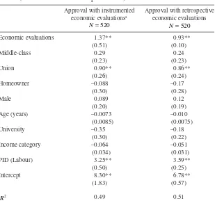
Table 2. Instrumental Variables (SLS) Estimates of Cross-Sectional Model (robust standard errors in parentheses)

Approval with instrumented

a_{Economic evaluations instrumented with current and change values of major purchase and} included exogenous variables.

**p < .01

(13)

We can now test whether or not the instruments are correlated with the error term. Specifically, we use Wooldridge’s heteroskedasticity-robust score test of overidentifying restrictions. The null hypothesis is that the instruments are uncorrelated with the error term. This is the second of the IV assumptions and

is known as an exclusion restriction (Wooldridge 2006, 525). The score test has

a chi-square distribution (chi2_{(1) = 0.76;}_p_{= 0.38). The score indicates that we}

cannot reject the null hypothesis that the instruments are uncorrelated with the

error term.14

The difficulty with this or any test of the exclusion restriction is that when the instruments pass the overidentification test, it could very well mean the instruments are uncorrelated with the error term (they are exogenous), but there does remain the possibility that the instruments pass this test because both instruments are endogenous in a way that produces biases of the same

magnitude (Wooldridge 2002). This is a real difficulty with cross-sectional

data and is one of the elements in the compelling argument made by some that an instrument is rarely convincing outside experimental randomization (e.g., Savoy and Green 2008). However, much can also be done with longitudinal

data to support our overidentification test.15

If one instrument is convincingly exogenous, the overidentification test will not have the above weakness. Our two instruments are major purchase and the change in major purchase. The potential sources of endogeneity for our instruments are equivalent to those for the original economic evaluation vari-able: (1) the instrument is predicted by a lag of government approval; (2) the instrument is predicted by fixed characteristics of individuals that also predict government approval; (3) the instrument is predicted by omitted time-varying variables; or (4) the instrument is caused by government approval (reverse causation). As we demonstrate when we present the solution 2 results below, we can use the panel data to demonstrate that changes in major purchase are independent of changes in government approval. Thus, the change instrument is unlikely to be endogenous to government approval due to any time-varying omitted variables (endogeneity problem 3) or reverse causation (problem 4). Since the instrument represents a change in the individuals’ opinions, it is also unlikely to be endogenous due to any fixed characteristics (problem 2). These elements are differenced out in the major-purchase change variable. Further, we use the panel data to demonstrate that change in major purchase is not pre-dicted by a lag of government approval and so will not be endogenous due to the exclusion of the lag of government approval in model 4 (problem 1). These facts provide substantial support for our contention that the major-purchase change instrument is exogenous and that the results of the overidentification test indicate that the major-purchase variable is also exogenous.

14. Further tests of the major-purchase variable as an instrument are included in the online appen-dix, section A.6.

15. Savoy and Green (2008) do suggest that a lag of a variable might be a convincing instrument.

(14)

Having rejected the null hypothesis that the major-purchase variables are weak instruments and having not rejected the null hypothesis that the instruments are uncorrelated with the error term, we can proceed with interpreting the results from the IV estimation. Economic evaluations are estimated on a five-point scale, and government approval on a ten-point scale. The effect of a one-unit difference in economic evaluations is a 1.37-unit difference in government approval.

Table 2 also presents the results of estimating the same model without instrumenting retrospective economic evaluations. We would still have found their effect to be statistically significant but would have concluded that they are smaller in magnitude. The discrepancy is probably because our instrumen-tal variables are effective at filtering measurement error noise out of the

eco-nomic evaluations measure (Wooldridge 2002, 95). The noise may be creating

attenuation bias in the OLS estimation of the model based on equation (4). We now examine solution 2 with the application of the Lancaster likelihood-based approach to estimating the parameters in a panel model likelihood-based on equation

(1).16_{This estimates the effects of changes in economic evaluations within}

individ-uals. To allow for the potential of a common trend across all cases, as indicated by

τ_t in equation (3), we explicitly estimate these parameters. We originally included

a nonlinear trend by allowing for a different intercept in each wave (including τ

2

and τ_{3 with wave one as the control) but found that the results are indistinguishable}

from using a linear trend (including τ

2 and 2Xτ2 with wave one as the control).

These estimates are presented in the first two columns of table 3.

The results indicate that individual changes in economic evaluations did have a statistically significant and positive effect on government approval

from 2009 until the 2010 general election.17_{However, these results control}

only for endogeneity problems 1 and 2. To control for endogeneity problems 3

and 4, we instrument retrospective economic evaluations.18

The results of instrumenting retrospective economic evaluations in our panel

data model are presented in the third column of table 3. Before interpreting the

results, we examine the strength of the instrumental variable in the panel setting. From the model estimation, we get individual tests of the null hypothesis that the instrument does not predict retrospective economic valuations in each wave (see the online appendix, section A.6). In all three waves, we can reject the null hypoth-esis. The instruments correlate in a significant way with the instrumented variable. As indicated in the presentation of the solution 1 results, we can also test the extent to which changes in our instrument are determined by government approval by estimating a panel model equivalent to equation (2)—assuming

16. As the Lancaster approach is essentially Bayesian, it was straightforward to incorporate the imputation of missing values from all variables with the observed values from the same variables from other waves. For missing data values, imputed values are drawn from the posterior distribu-tion of the variables condidistribu-tioning on the observed values from the other periods.

17. The online appendix, section A.7, includes estimates of the model based on (2) using the Lancaster likelihood-based approach

18. The online appendix, section A.2, provides detail on the estimation approach.

(15)

Table 3. Likelihood-Based Estimates of Panel Models†

DIC 2275740 2275740 2281550 2269090 2269090

†_{These are Bayesian estimates derived using MCMC methods. The reported coefficients represent the medians of the posterior distributions. The standard}

devia-tions of the posterior distribudevia-tions are in parentheses. *p < .05; **p < .01

749

(16)

first k₌0_{and second}k₌₁_{—substituting the major-purchase variable for the} retrospective economic evaluation variable. The results are presented in the

last two columns of table 3.

The results indicate that within-individual changes in major-purchase evaluations are not determined by within-individual changes in government approval and that within-individual changes in major-purchase evaluations are not determined by past (lag of) major-purchase evaluations. Recall that this has important implications for solution 1. The first result provides strong sup-port for the claim that the change instrument is not endogenous to government approval due to any time-varying omitted variables or reverse causation. The second result indicates that that the change instrument will not be endogenous due to any correlation with the lag of government approval.

Turning back to solution 2, these results demonstrate the importance of con-trolling for all forms of endogeneity and the value of our instrumental variable. The estimated effect of economic evaluations on government approval, once

eco-nomic evaluations are instrumented, drops to statistical insignificance (table 3,

column 3). Not only is the effect statistically insignificant, but the estimated coef-ficient is less than one-twentieth the magnitude of the non-instrumented estimate.

Discussion

We have identified sources of endogeneity and specified solutions that can appropriately address them. Our first solution introduced the use of an instru-mental variable approach to reduce bias and noise/measurement error when estimating the effect of differences in economic evaluations between individu-als in cross-sectional data. However, the effect of differences between individ-uals is only one potentially observable implication of economic voting theory. When an individual’s evaluation of the economy changes, their support for the incumbent party is also expected to change. Identifying this effect requires panel data, and thus the second solution introduced the likelihood-based

esti-mation of a panel model developed by Lancaster (2002). The estimated panel

model provides a useful estimate of endogeneity-purged economic effects that deal with source of endogeneity 1 and 2. Although endogeneity problem 3 can also be reduced using this method through the addition of relevant dynamic variables in model (1), it cannot resolve endogeneity problem 4. Therefore, we proposed that the likelihood-based estimation of the panel model be used in conjunction with the instrument for subjective economic evaluations, thereby also addressing endogeneity problems 3 and 4.

On the basis of this analysis, it appears that responses to the “major pur-chase” question serve to isolate those aspects of a respondent’s retrospective economic evaluations that are actually driven by economic performance from those that derive from factors such as partisan conditioning. Our instrument passes the usual test of being a strong instrument and being uncorrelated with Pickup and Evans 750

(17)

the model errors, whether modeling cross-sectional differences or over-time changes in government approval. We also go further than the usual cross- sectional tests by using the availability of panel data to demonstrate the valid-ity of our instrument.

Our use of an Internet panel leaves open the generalizability of these find-ings to the general population, though it is unlikely to do so any more than any other panel, plagued as all panels are by attrition that weakens their repre-sentativeness with respect to, typically, less politically interested respondents. Moreover, as reported in the online appendix, section A.3, the validation exer-cises conducted on the YouGov procedures indicate equivalent voting model parameters to those obtained from a cross-sectional face-to-face random

sam-ple (Sanders et al. 2007).

What implications does our analysis have for understanding the impact of economic evaluations on government approval and, ultimately, voting? We have seen that the application of the instrumental variable method to cross-sectional data indicates that long-term differences in economic evaluations between individuals do have an effect that is not endogenous. The estimated

effect is similar to that of others using subjective economic indicators (van der

Eijk et al. 2007; Duch and Stevenson 2008). Using the instrumental variable in conjunction with Lancaster’s orthogonal re-parameterization likelihood-based

estimation procedure with panel data indicates that short-term changes in the

economic evaluations of individuals do not have an exogenous effect. This is

consistent with other panel data estimates of within-individual effects (Evans

and Andersen 2006; Evans and Pickup 2010). These results resolve the differ-ences in the findings across these studies. Economic evaluations do matter, but short-term changes in those evaluations do not. If and when we have compara-ble panel data for a longer period of time, we may well find that changes in the long term do have an exogenous effect on government support. Until then, we can conclude that voters are not responding to the small ripples in their evalu-ations of the economy, but it remains to be seen whether or not they respond to the long-term tide of economic sentiment.

Appendix. Question Wording

In addition to the sociotropic, retrospective economic evaluation question mentioned in the text, the following questions were asked as part of the British Cooperative Campaign Analysis Project survey.

Governing Party Approval

On the scale below, please indicate how you feel about the Labour Party.

0 < Unfavorable; 10 > Favorable; Don’t know.

Major Purchase

In view of the general economic situation, do you think now is the right time for people to make major purchases, such as furniture or electrical goods?

(18)

Now is the right time for people to make a major purchase; Now is neither the right nor the wrong time for people to make a major purchase; Now is the wrong time for people to make a major purchase.

Homeowner

Which of the following best describes your homeownership status?

Own outright; Own with a mortgage; Rent from a private landlord; Rent from a local authority/housing association; Other; Don’t know.

Partisan Identification

Generally speaking, do you think of yourself as Labour, Conservative, Liberal Democrat, or what?

Labour; Conservative; Liberal Democrat; Scottish National Party (SNP); Plaid Cymru; Green Party; United Kingdom Independence Party (UKIP); British National Party (BNP); Other; None; Don’t know.

Education, union membership, gender, and class were recorded previously by YouGov.

Supplementary Data

Supplementary data are freely available online at http://poq.oxfordjournals.org/.

References

Anderson, Christopher J. 2007. “The End of Economic Voting? Contingency Dilemmas and the Limits of Democratic Accountability.” Annual Review of Political Science 10:271–96. Anderson, Christopher J., Silvia M. Mendes, Yuliya V. Tverdova, and Haklin Kim. 2004.

“Endogenous Economic Voting: Evidence from the 1997 British Election.” Electoral Studies 23:683–708.

Angrist, Joshua D., and Alan B. Krueger. 2001. “Instrumental Variables and the Search for Identification: From Supply and Demand to Natural Experiments.” Journal of Economic Perspectives 15:69–85.

Arellano, Manuel. 2003. Panel Data Econometrics. Oxford, UK: Oxford University Press. Arellano, Manuel, and Stephen Bond. 1991. “Some Tests of Specification for Panel Data: Monte

Carlo Evidence and an Application to Employment Equations.” Review of Economic Studies 58:277–97.

Bartels, Larry, M. 2002. “Beyond the Running Tally: Partisan Bias in Political Perceptions.” Political Behavior 24:117–50.

Curran, Patrick J., and Daniel J. Bauer. 2011. “The Disaggregation of Within-Person and Between-Person Effects in Longitudinal Models of Change.” Annual Review of Psychology 62:583–619. Deming, W. Edwards. 1985. Statistical Adjustment of Data. Dover, UK: John Wiley and Sons. Duch, Raymond M., Harvey D. Palmer, and Christopher J. Anderson. 2000. “Heterogeneity in

Perceptions of National Economic Conditions.” American Journal of Political Science 44:635–52. Duch, Raymond M., and Randy Stevenson. 2008. Voting in Context: How Political and Economic

Institutions Condition Election Results. Cambridge, UK: Cambridge University Press. Engle, Robert F., David F. Hendry, and Jean-François Richard. 1983. “Exogeneity.” Econometrica

51:277–304.

Enns, Peter, Paul Kellstedt, and Gregory McAvoy. 2012. “The Consequences of Partisanship in Economic Perceptions.” Public Opinion Quarterly 76:287–310.

(19)

Erikson, Robert S. 1989. “Economic Conditions and the Presidential Vote.” American Political Science Review 83:567–83.

Erikson, Robert S., Michael B. MacKuen, and James A. Stimson. 2002. The Macro Polity. New York: Cambridge University Press.

Evans, Geoffrey, and Robert Andersen. 2006. “The Political Conditioning of Economic Perceptions.” Journal of Politics 68:194–207.

Evans, Geoffrey, and Mark Pickup. 2010. “Reversing the Causal Arrow.” Journal of Politics 72:1236–51.

Fiorina, Morris. 1981. Retrospective Voting in American National Elections. New Haven, CT: Yale University Press.

Gerber, Alan S., and Gregory A. Huber. 2009. “Partisanship and Economic Behavior: Do Partisan Differences in Economic Forecasts Predict Real Economic Behavior?” American Political Science Review 103:407–26.

Golinelli, Roberto, and Giuseppe Parigi. 2003. “What is this thing called confidence? A compara-tive analysis of consumer confidence indices in eight major countries.” Temi di discussione (Economic working papers) 484, Bank of Italy, Economic Research and International Relations Area.

Greene, William H. 2003. Econometric Analysis. 5th ed. Englewood Cliffs, NJ: Prentice Hall. Hendry, David. 2003. Dynamic Econometrics. Oxford, UK: Oxford University Press.

Hetherington, Marc. 1996. “The Media’s Role in Forming Voters National Economic Evaluations in 1992.” American Journal of Political Science 40:372–95.

Kinder, Donald R., and D. Roderick Kiewiet. 1981. “Sociotropic Politics: The American Case.” British Journal of Political Science 11:129–61.

Ladner, Matthew, and Christopher Wlezien. 2007. “Partisan Preferences, Electoral Prospects, and Economic Expectations.” Comparative Political Studies 40:571–96.

Lancaster, Tony. 2002. “Orthogonal Parameters and Panel Data.” Review of Economic Studies 69:647–66.

Lewis-Beck, Michael S., and Mary Stegmaier. 2007. “Economic Models of the Vote.” In The Oxford Handbook of Political Behavior, edited by Russell Dalton and Hans-Dieter Klingemann, 518–37. Oxford, UK: Oxford University Press.

Lillard, Lee, and Robert Willis. 1978. “Dynamic Aspects of Learning Mobility.” Econometrica 46:985–1012.

Marsh, Michael, and James Tilley. 2010. “The Attribution of Credit and Blame to Governments and Its Impact on Vote Choice.” British Journal of Political Science 40:115–34.

Neyman, Jerzy, and Elizabeth L. Scott. 1948. “Consistent Estimation from Partially Consistent Observations.” Econometrica 16:1–32.

Raudenbush, Stephen. 2001. “Comparing Personal Trajectories and Drawing Causal Inferences from Longitudinal Data.” Annual Review of Psychology 52:501–25.

Rehm, Philipp. 2009. “Risks and Redistribution: An Individual-Level Analysis.” Comparative Political Studies 42:855–81.

Rudolph, Thomas. 2003. “Who’s Responsible for the Economy? The Formation and Consequences of Responsibility Attributions.” American Journal of Political Science 47:698–713.

Sanders, David, Harold D. Clarke, Marianne C. Stuart, and Paul Whiteley. 2007. “Does Mode Matter for Modeling Political Choice? Evidence from the 2005 British Election Study.” Political Analysis 15:257–85.

Sanders, David, and Neil. T. Gavin. 2004. “Television News, Economic Perceptions, and Political Preferences in Britain, 1997–2001.” Journal of Politics 66:1245–66.

Savoy, Alison, and Donald Green. 2008. “Instrumental Variables Estimation in Political Science: A Readers’ Guide.” American Journal of Political Science 55:188–200.

Tilley, James, and Sara Hobolt. 2011. “Is the Government to Blame? An Experimental Test of How Partisanship Shapes Perceptions of Performance and Responsibility.” Journal of Politics 73:316–30.

(20)

van der Eijk, Cees, Mark N. Franklin, Froukje Demant, and Wouter van der Brug. 2007. “The Endogenous Economy: ‘Real’ Economic Conditions, Subjective Economic Evaluations, and Government Support.” Acta Politica 42:1–22.

Wilcox, Nathaniel, T., and Christopher Wlezien. 1993. “The Contamination of Responses to Survey Items: Economic Perceptions and Political Judgments.” Political Analysis 5:181–213. Wlezien, Christopher, Mark Franklin, and Daniel Twiggs. 1997. “Economic Perceptions and Vote

Choice: Disentangling the Endogeneity.” Political Behavior 19:7–17.

Wooldridge, Jeffrey M. 2002. Econometric Analysis of Cross-Sectional and Panel Data. 2nd ed. Cambridge, MA: MIT Press.

———. 2006. Introductory Econometrics: A Modern Approach. 3rd ed. Mason, OH: Thompson South-Western.