IJOG
A Drowning Sunda Shelf Model during Last Glacial Maximum (LGM)
and Holocene: A Review
Tubagus Solihuddin
Center for Research and Development of Marine and Coastal Resources Jln. Pasir Putih 1, Ancol Timur, Jakarta 14430
Corresponding author: [email protected]
Manuscript received: April 14, 2014, revised: July 16, 2014, approved: August 15, 2014
Abstract - Rising sea levels since the Last Glacial Maximum (LGM), some ~20,000 years ago, has drowned the
Sunda Shelf and generated the complex coastal morphology as seen today. The pattern of drowning of the shelf will be
utilized to assess likely timing of shoreline displacements and the duration of shelf exposure during the postglacial sea
level rise. From existing sea level records around Sunda Shelf region, “sea level curve” was assembled to reconstruct the shelf drowning events. A five stage drowning model is proposed, including 1) maximum exposure of the shelf at approximately 20,500 years Before Present (y.B.P.), when sea level had fallen to about -118 m below present sea level (bpl.), 2) melt water pulse (MWP) 1A at ~14,000 y.B.P. when sea level rose to about -80 m bpl., 3) melt water pulse (MWP) 1B at ~11,500 y.B.P., when sea level was predicted around -50 m bpl., 4) Early-Holocene at ~9,700 y.B.P, when sea level was predicted at about-30 m bpl, and 5) sea level high stand at ~4,000 y.B.P., when sea level jumped to approx. +5 m above present sea level (apl.). This study shows that the sea level fluctuated by more than 120 m at various times during LGM and Holocene. Also confirmed that sea level curve of Sunda Shelf seems to fit well when combined with sea level curve from Barbados, although the comparison remains controversial until now due to the considerable distinction of tectonic and hydro-isostatic settings.
Keywords: Last Glacial Maximum, sea-level changes, transgression, drowning shelf
Introduction
The Sunda Shelf is located in Southeast Asia
and it represents the second largest drowned continental shelf in the world (Molengraaff and
Weber, 1921; Dickerson, 1941). It includes parts of Indonesia, Malaysia, Singapore, Thailand, Cambodia, Vietnam coast, and shallow seabed of the South China Sea (Figure 1). During the LGM, when sea levels are estimated -116 m be
-low present sea level (bpl.), the Sunda Shelf was
widely exposed, forming a large land so-called
“Sunda Land” connecting the Greater Sunda Islands of Kalimantan, Jawa, and Sumatra with
continental Asia (Geyh et al., 1979; Hesp et al.,
1998; Hanebuth et al., 2000, 2009).
The Sunda Shelf is also considered as a tectonically stable continental shelf during the Quaternary (Tjia and Liew, 1996) and categorized as a “far field” location (far away from former ice sheet region), providing the best example for observing sea level history and paleo-shoreline
reconstruction. In such environment, the effects
of seafloor compaction, subsidence, and
hydro-isostatic (melt water release from the ice sheets)
compensation are negligible during the relatively
short time interval of thousands of years
(Lam-beck et al., 2002; Wong et al., 2003).
This study reviews some published sea level observations then presenting a summary of the Sunda Shelf drowning model. Moreover, it dis -cusses some sea level records from different
lo-INDONESIAN JOURNAL ON GEOSCIENCE
Geological Agency
Ministry of Energy and Mineral Resources
IJOG
calities in time-scale LGM to Holocene (Table 1)and improves detailed colour maps of Holocene sea level transgression on the Sunda Shelf (Voris, 2000; Sathiamurthy and Voris, 2006) in terms of
map resolution. The analyses and data presented in this paper provide an up to date overview of the history of sea level and paleo-shoreline changes
around Sunda Shelf region since the LGM to Holocene.
Reconstructing Sea-level History
Studies on sea level history around Sunda Shelf have been carried out by Geyh et al., (1979), Tjia, (1996), Hesp et al., 1998, and Hanebuth et al., (2000, 2009) to provide information on
paleo-shoreline, paleo-river, and paleo-bathymetry. The most relatively recent studies (Hanebuth et al., 2000, 2009) demonstrated an important
Figure 1. A map shows the Sunda Shelf region derived from 30 arc-seconds resolution bathymetric grid sourced from GEB
-CO. (after Molengraaff and Weber, 1921; Dickerson, 1941).
3000 m
-5000 m
-7250 m
0 500
N
1000 Kilometre
2500 m
-2500 m 0 m
Kalimantan
Sum atra
Sahul S helf Thailand
Sunda Shelf
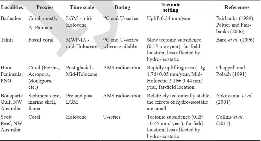
Table 1. Sea Level Observations from some Localities presenting LGM - Holocene Sea-level Records
Localities Proxies Time scale Dating Tectonic
setting References
Barbados Coral, mostly A. Palmata
LGM -
mid-Holocene
14C and U-series Uplift 0.34 mm/year Fairbanks (1989), Peltier and
Fair-banks (2006)
Tahiti Fossil coral MWP-IA -
mid-Holocene
14C and U-series
where available Slow tectonic subsidence (0.15 mm/year), far-field location, less affected by
hydro-isostatic
Bard et al. (1996)
Huon
Peninsula, PNG
Coral (Porites, Acropora, Montipora, etc.)
Post glacial -
Mid-Holocene AMS radiocarbon Rapidly uplifting area (LIg 1.76±0.05 mm/year,
Mid-Holocene 2.16± 0.44 mm/ year, far-field location
Chappell and Polach (1991)
Bonaparte
Gulf, NW
Australia
Sediment core,
marine shell, fauna
Pre and post LGM
AMS radiocarbon Relatively tectonically stable,
the effects of hydro-isostatic are small
Yokoyama et al. (2001)
Scott Reef, NW
Australia
Coral Holocene U-series Tectonic subsidence (0.29
- 0.45 mm/ year), far-field location, less affected by
hydro-isostatic
IJOG
recent dataset from a number of sediment coreswhich were dated by AMS radiocarbon, providing records extending from LGM to Holocene that fill some of the late-Glacial gaps from Barbados records. The Sunda Shelf region is believed to have been tectonically stable during the Pleistocene (Tjia and Liew, 1996) and considered as a “far-field” site where tectonic correction and hydro-isostatic compensation are negligible.
The stages of rising sea levels on the Sunda Shelf between ~21,000 y. B.P. and ~4,200 y. B.P. were reported by Hanebuth et al. (2000). It was
initiated by the terminal phase of LGM sea level lowstand (approximately -116 m bpl.) at about 21,000 y. B.P. and followed by transgression, rising sea level to approx. -56 m bpl. at ~11,000 y. B.P. Whilst Geyh et al. (1979), Tjia (1996), and Hesp et al. (1998) described the sea level
highstand and its gradual fall to current levels
thereafter in the Mid to Late Holocene. The summary is as follows. In the EarlyHolocene between 10,000 and 6,000 y. B.P., the sea levels rose significantly from -51 m bpl. to 0 m (present
level). Following this, it reached a peak in the
Mid-Holocene between 6,000 and 4,200 y. B.P., exhibiting sea level highstand from 0 m to +5m
apl. After that, the sea level fell gradually until
reaching modern sea level at about 1,000 y. B.P.
(Figure 2).
Materials and Methods
The ocean topography and land data covering
the Sunda Shelf were extracted from the General Bathymetric Chart of the Ocean Grid (Gebco) 0.8
grid with a spatial resolution of 30 arc-seconds of latitude and longitude (1 minute of latitude =
1.853 km at the equator). The bathymetric grid has largely been generated from a database of over 290 million bathymetric soundings with interpolation between soundings guided by
satellite-derived gravity data. Land data are
largely based on the Shuttle Radar Topography Mission (SRTM30) gridded digital elevation model (see web page at: http://www.gebco.net/ data and products/gridded bathymetry data/; ac -cessed July 2013).
The extracted elevation data (in x, y, and z
coordinates) were exported into points in ASCII
format within GridViewer package programme. These point data were then used to generate a
Digital Elevation Model (DEM) using a Trian -gulated Irregular Network (TIN) method or TIN
DEM within the Global Mapper v11.0 toolkit.
For the purpose of a two-dimensional layout, a
Grid DEM was generated and presented within MapInfo7.0 software. All figures presented on this paper are originally created by the author following the method discussed above.
The sea-level curve estimation in Sunda Shelf as shown in Figure 2 is derived from some
previous studies conducted in several localities
such as Strait of Malacca (Geyh et al., 1979),
Singapore (Hesp et al., 1998), and former North Sunda River and Mekong Delta (Hanebuth et
al., 2000, 2009). This sea-level curve was then
correlated with the present-day topography
and bathymetry of the Sundaland to generate maps and approximate shoreline configuration of the Sundaland during the latest Quaternary. However, several assumptions were made in the workflow of this study as follows: 1) The current topography and bathymetry of the Sunda Shelf are only an approximation and do not reflect past condition precisely. 2) The sea floor compaction, subsidence, and vertical crust displacement due to
sedimentation, scouring, and tectonic processes are not taken into account.
Geyh et al., (1979)
Relative Sea Level (m)
-100
-120
-140
0 5000
14
Time ( C calibrated years BP)
10000 15000 20000 25000 0
Hesp et al., (1995) Hanebuth et al., (2000) Hanebuth et al., (2009) Regression line order 3
LGM lowstand Transgression
Holocene highstand
Figure 2. The best-fit sea level curve estimation of Sunda Shelf
from 21,000 to 1,000 y. B.P. derived from Geyh et al., (1979),
IJOG
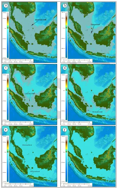
MapsThe maps presented in this paper show a
summary of the gradual Sunda Shelf drowning
model which represents the predicted shorelines
and shelf exposures during LGM and Holocene. Starting from -118 m depth contour, the drowning model was gradually established on a vertical el
-evation of -80 m, -50 m, -30 m, +5m, and present
sea-level which every depth contour corresponds to 14C calibrated years Before Present age. For example, the current -118 m depth contour was
predicted as a shoreline at approx. 20,500 y. B.P., while the current -50 m depth contour was
attributed to 11,500 y. B.P., etc. Topographic and bathymetric contours are indicated by the change in colour scheme as shown in the legend; how
-ever, the grey colour is also applied to the DEM
representing the exposed shelf. In addition, the
flowage of paleo-river of Sunda Shelf during
LGM is also presented with refers to the map
of paleo-river (Voris, 2000; Sathiamurthy and
Voris, 2006).
Results
The Drowning Sunda Shelf History
The history of the drowning Sunda Shelf was
initiated at approximately 20,500 y. B.P. when sea
level had fallen to around -118 mbpl. By this time, the Sunda Shelf was largely exposed, forming
a massive lowland which connects present-day
mainlands in this region (Kalimantan, Jawa, Su -matra, and Malaya Peninsula) (Figure 3a).
Dur-ing melt water pulse (MWP)-1A, some ~14,000 y. B.P. (Fairbank, 1989), sea level rose rapidly to approx. -80 m bpl., inundating Sunda Shelf around the present-day Natuna Island. However,
the mainlands were still connected to each other
and the configuration of the exposed Sunda Shelf remained very similar to the -118 m bpl. forma
-tion (Figure 3b).
Following that, the sea-level still experienced
a rapid rise and jumped to around -50 m bpl. at about 11,500 y. B.P. (MWP-1B of Fairbank, 1989), exhibiting initial isolation of Natuna and the Anambas Islands from the mainland. Thus, the connections between Kalimantan and Malaya Peninsula via South China Sea were initially
separated. Adding that, the present-day Jawa Sea,
which connects Kalimantan and Jawa, was largely inundated, separating partly the two mainlands
(Figure 3c). However, the Greater Sundaland
(i.e. Kalimantan, Jawa, and Sumatra) were still connected to the Malaya Peninsula.
At approx. 9,700 y. B.P., when sea level was
predicted around-30 m bpl., the Jawa Sea became a significant sea. The present-day Sunda , Kari
-mata , and Malacca Straits, the land bridges that connect the Greater Sundaland, were initially
inundated, forming a narrow channel among the islands (Figure 3d). The marine transgression
reached a peak in the Mid-Holocene at approx. 4,000 y. B.P., rising sea level to about +5 m apl.
and drowning some lowland areas in the mainland (Figure 3e). Finally, the sea level fell gradually returning to present-day level at approx. 1,000 y. B.P. (Figure 3f).
Paleo-rivers on the Sunda Shelf
There were four large river systems on the
Sunda Shelf that drained the Sundaland dur
-ing the LGM; the Siam River, the North Sunda River, East Sunda River, and the Malacca Strait River systems (Voris, 2000) (Figure 4). The Siam
River system which today is called Chao Phraya included the river system of east coast of Malaya
Peninsula (Sungai Endau, Sungai Pahang, Sungai Terengganu, and Sungai Kelantan) and part of the Southwest Vietnam coast. Sathiamurthy and Voris (2006) demonstrated that Sumatra’s Sun
-gai Kampar also joined the Siam River system through the Singapore Strait and then ran north to the Gulf of Thailand where the major Siam River
system situated and drained to the large expanse
of Sunda Shelf.
The North Sunda River system was considered as the major Sunda Shelf River system (Mo
-lengraaff Rivers of Dickerson, 1941; Kuenen, 1950; Tjia, 1980) which drained north to the sea
northeast of Natuna Island. This system included
some tributaries of Central and South Sumatra coast (Sungai Indragiri, Sungai Batanghari, and Sungai Musi) and the large Kapuas River system
from Kalimantan.
The East Sunda River system drained to the east across what is the present-day Jawa Sea be
IJOG
3000 m
-5000 m
-7250 m
0 km 250 km 500 km 750 km 1250 km
2500 m
-2500 m 0 m 3000 m
3000 m 3000 m
3000 m 3000 m
-5000 m
-5000 m -5000 m
-5000 m -5000 m
-7250 m
-7250 m -7250 m
-7250 m -7250 m
0 km
0 km 0 km
0 km 0 km
250 km
250 km 250 km
250 km 250 km
500 km
500 km 500 km
500 km 500 km
750 km
750 km 750 km
750 km 750 km
1250 km
1250 km 1250 km
1250 km 1250 km
2500 m
2500 m 2500 m
2500 m 2500 m
-2500 m
-2500 m -2500 m
-2500 m -2500 m
0 m
0 m 0 m
0 m 0 m
Figure 3. Shelf and sea level exposures at various ages. a). 20,500 y BP, sea level of - 118 m bpl. b). 14,000 y BP (MWP 1A), sea level of - 80 m bpl. c). 11,500 y BP (MWP 1B), sea level - 50 m bpl. d). 9,700 y BP, sea level of - 30 m bpl-pre
-dicted. e). 4,000 y BP, sea level +5 m apl. f). Present day sea level. Map derived from 30 arc-seconds resolution bathymetric grid sourced from GEBCO.
a
b
c
d
IJOG
Mekong Chao
Malacca Strait River
Sumatra Sunda Shelf
E. Sunda River
Kalimantan
Jawa
0 250
Kilometre 500
N
Malaysia
N. Sunda River
Figure 4. A map shows paleo-rivers on the Sunda Shelf during LGM (After Voris, 2000; Sathiamurthy and Voris,
2006).
included present-day rivers of north coast of Jawa, the south coast of Kalimantan and the northern
portion of the east coast of Sumatra. Some smaller rivers in SE Sumatra and the Seribu Islands area of Jawa Sea ran south via the Sunda Strait to enter the Indian Ocean (Umbgrove, 1949; van
Bemmelen, 1949).
The Straits of Malacca River system had two drainages separated by a topographic height between the Bernam and Kelang Rivers. One drained NW to the Andaman Sea, including some tributaries of this river system i.e. Sungai Sim
-pang Kanan, Sungai Panai, Sungai Rokan, and Sungai Siak of east coast of Sumatra and some
rivers from the west coast of Malaya Peninsula
i.e. Sungai Perak, Sungai Bernam, Sungai Muar, and Sungai Lenek. Whilst the other drained SW and eventually joined the North Sunda River.
Discussion
Comparison with Data from other Studies Some studies have been carried out from dif
-ferent localities to obtain sea-level stands during LGM and Holocene. The observations resulted in
varied conclusions depending mainly on covering time periods, proxies, dating methods, isostatic effects, and vertical tectonic land movement.
Hence, it is necessary to consider those men
-tioned factors when combining the data into a
single dataset and generating sea level curve on these data. Also, when comparing these sea-level
records to Sunda Shelf data, those factors should be taken into account to avoid bias in analysis
and interpretation.
Fairbanks (1989) and Peltier and Fairbanks
(2006) reported an important source of
informa-tion for relative sea-level changes in Barbados
during the late stages of the LGM and the late-Glacial period. Using coral cores as a proxy and
AMS radiocarbon calibrated by Thermal Ionisa
-tion Mass Spectrometry (TIMS) dating methods, the local relative sea level in Barbados stood between -125 m bpl. at 21,000 y. B.P. and -15 m bpl. at 7,000 y. B.P. (Figure 5). The uplift rate
was 0.34 mm/year due to local tectonic setting. Meanwhile, the relative sea-level change data
in Tahiti is from Bard et al., (1996) with
sup-porting information on coral species given by
Montaggioni and Gerrard (1997). Using coral as
a proxy, radiocarbon dating yielded time scale between MWP-1A and Mid-Holocene (Figure 5). Tahiti experienced slow tectonic subsidence
(0.15 mm/year) and was also characterized as a
“far-field” location.
The local relative sea-level changes were also investigated from a rapidly uplifting area such as
Huon Peninsula, Papua New Guinea. The records were obtained from a raised Holocene reef drill core collected by Chappell and Pollach (1991). AMS radiocarbon dating was applied to the
samples and uranium series (U-series) ages were
subsequently obtained from the same samples by Edward et al. (1993), providing sea-level
indica-tors from post-Glacial to Mid-Holocene (Figure
5). The uplift rate was reported 1.76 ± 0.05 mm/ year in the last-Interglacial (LIG) and 2.16 ± 0.44
mm/year in the Mid-Holocene. This region was also considered as a “far-field” location.
Moreover, Yokoyama et al. (2001) discussed
the relative sea-level estimation from the NW Australia Shelf. The information was obtained
from the sediment cores of Bonaparte Gulf which
were dated by AMS radiocarbon dating, providing
sea-level indicators corresponding to a late stage
IJOG
and was considered as a “far-field” site where theeffects of hydro-isostatic are small.
The most relatively recent studies (Collins
et al., 2011) demonstrated an important recent
dataset from a number of coral cores in Scott Reef, Northwest Australia, which were dated by
high resolution U-series dating. The data provided
Holocene sea-level records that characterized by
moderate rates of sea-level rise of 10 mm/year and
confirmed tectonic subsidence of 0.29 - 0.45 mm/ year (Figure 5). The region was also less affected
by hydro-isostatic due to “far-field” location. Despite the fact that Sunda Shelf and NW
Australia region are proximal and considered to
be tectonically stable at least during Holocene and less affected by glacio-isostatic adjustment due to their ‘far-field’ locations, the sea level curve of Sunda Shelf during LGM and Holocene seems to fit well when combined with sea level curves from Barbados. This is also in accordance with Peltier and Fairbanks (2006) who reported that the com
-bination between Bonaparte Gulf, NW Australia,
and Sunda Shelf records did not match together well and suggested that Sunda Shelf records fit much better with the Barbados dataset. However, the tectonic and hydro-isostatic settings of Sunda Shelf and Barbados differ considerably and that
comparison remains controversial until now.
Sea-level High Stand during Mid-Holocene and There after
Another issue that arises in the discussion of
the Sunda Shelf sea-level history is the contro
-versy of the precise details of the Mid-Holocene highstand. The dispute is likely because of the variation on timing, glacio-isostatic adjustment,
and localised tectonics. For example, one
ap-praisal of evidence from Malay-Thai Peninsula
(Tjia, 1996) revealed that the sea level highstand
peaked at +4 m at 6,000 y. B.P. and +5 m at 5,000
y. B.P. Whilst, an earlier survey in the Strait of Malacca, between Port Dickson and Singapore
(Geyh et al., 1979) evidenced the highest dated
level at +2.5 m to about +5.8 m for the time inter
-U/Th Barbados coral (Fairbanks, 1989) 20
0
0 5 10 15 20 25 35
-20
-40
-60
-80
-100
-120
-140
-160
14C Tahiti coral (Bard et al., 1996)
14C Huon Peninsula coral (Chappell and
Polach, 1991)
14C Bonaparte Gulf sediment core
(Yokoyama et al., 2001)
U/Th Scott Reef coral (Collins et al., 2011)
Best-fit-sea-level curve for Barbados
Best-fit-sea-level curve for Tahiti
Best-fit-sea-level curve for Scott Reef
Age (x1000 calibrated y BP)
Relative sea-level (m)
Best-fit-sea-level curve for Baonaparte Gulf
Best-fit-sea-level curve for Huon Peninnsula
IJOG
val between 5,000 and 4,000 y. B.P. Furthermore,review from two areas in Singapore, Sungai Nipah, and Pulau Semakau (Hesp et al., 1998) concluded that the peak of the sea level at about +3 m rather than +5 m between 6,000 y. B.P. and 3,500 y. B.P.
Despite such discrepancies, there is a general
consensus (Geyh et al., 1979; Tjia, 1996; Hesp et
al., 1998) that the sea level highstand was attained by ~6,000 y. B.P. or slightly earlier. By that time, the sea level was around +3 m to +5 m above pres -ent sea-level then receded to its curr-ent datum for
the past ~1,000 years. The noticeable impact of sea
level rise through the transgression is that shore-line position changed markedly and was higher and landward of present level during the high
stand (~6,000 - 4,000 y. B.P.). As sea levels fell
post-highstand, the shoreline prograded seaward,
forming numerous beach ridges in the sequence.
Conclusions
The Sunda Shelf provides suitable environ -ments for sea level studies and has provided one
of the best examples of sea-level at the time of
the LGM. In particular, the continent is relatively
tectonically stable and lies far away from the for -mer ice sheets, thus the effects of hydro-isostatic
adjustment are less and eustatic changes should be well reflected in the data. The model reveals that the drowning Sunda Shelf was initiated at
~20,500 y. B.P., when sea level had fallen to
about -118 m bpl. During sea-level transgression, the Sunda Shelf experienced rapid sea-level rise,
inundating the shelf exposures until reaching
sea-level highstand at ~6,000 - 4,000 y. B.P.,
before finally returning to the present sea level at approx. 1,000 y. B.P. LGM and Holocene sea level changes are principally forced by the climate change; with sea level fluctuating by more than
120 m at various times. The trigger for these
climate and sea level variations is believed to relate to cyclic changes in the earth’s orbit and
solar radiation (the Milankovitch cycles) and the
insolation of the world’s atmosphere and oceans.
Acknowledgements
The author would like to thank Moataz Kordi, fellow PhD students at Curtin University, who
has helped a lot in map making and figures, also
productive discussions during reviewing an early draft of manuscript. The author also thanks to
Id-ham Effendi, researcher in Indonesian Geological
Agency, for his review of the manuscript and help
of the submission. This paper is a contribution to
Centre for Research and Development of Marine and Coastal Resources, Ministry of Marine Af-fairs and Fisheries.
References
Bard, E., Hamelin, B., Arnold, M., Montaggioni, L., Cabioch, G., Faure, G., and Rougerie, F.,
1996. Deglacial sea-level record from Tahiti
corals and the timing of global meltwater dis
-charge. Nature, 382(6588), p.241-244. doi:
p.10.1038/382241a0.
Chappell, J. and Polach, H., 1991.Post-glacial sea-level rise from a coral record at Huon
Peninsula, Papua New Guinea. Nature, 349(6305), p.147-149.
Collins, L. B., Testa, V., Zhao, J., and Qu, D.,
2011. Holocene growth history and evolution of the Scott Reef carbonate platform and coral
reef. Journal of the Royal Society of Western Australia, 94(2), p.239-250.
Dickerson, R. E., 1941. Molengraaff River: a
drowned Pleistocene stream and other Asian
evidences bearing upon the lowering of sea
level during the Ice Age. In: Speiser, E. A.
(ed.), Proceedings Universityof Pennsylvania, Bicentennial Conference, p.13-20. University of Pennsylvania Press.
Edwards, R. L., Beck, J. W., Burr, G. S., Donahue,
D. J.,Chappell, J. M. A., Bloom, A. L., Druffel,
E. R. M., and Taylor, F. W., 1993. A Large
Drop in Atmospheric 14C/12C and Reduced
Melting in the Younger Dryas, Documented with 230Th Ages of Corals. Science, 260
(5110), p.962-968.
Fairbanks, R. G., 1989. A 17,000-year glacio-eustatic sea level record influence of glacial
melting rates on the Younger Dry as event and deep ocean circulation. Nature, 342, p.637-642.
Geyh, M.A., Kudrass, H.R., and Streif, H., 1979.
-IJOG
cene and Holocene in the Strait of Malacca.
Nature, 278, p.441-443.
Hanebuth, T., Stattegger, K., and Grootes, P.M., 2000.Rapid Flooding of the Sunda Shelf:
A Late-Glacial Sea-Level Record. Science,
288(5468), p.1033-1035.
Hanebuth, T.J.J., Stattegger, K., and Bojanows
-ki, A., 2009. Termination of the Last Glacial
Maximum level lowstand: the Sunda
sea-level record revisited. In: Camoin, G.,
Drox-ler, A., MilDrox-ler, K., and Fulthorpe, C. (Eds.),
Records of Quaternary sea-level changes:
Global and Planetary Change, 66, p.76-84.
Hesp, P.A., Hung, C.C., Hilton, M., Ming, C.L.,
and Turner, I.M., 1998.A first tentative Holo
-cene sea-level curve for Singapore. Journal
of Coastal Research, 14, p.308-314.
Kuenen, P.H., 1950. Marine Geology. John
Wiley & Sons, Inc., New York, vii-568pp. Lambeck, K., Yokoyama, Y., and Purcel, A.,
2002. Into and out of the Last Glacial Maximum: sea-level change during Oxygen
Isotope Stages 3 and 2. Quaternary Science
Reviews, 21(1-3), p.343-360.
Molengraaff, G.A.F. and Weber, M., 1921. On the relation between the Pleistocene glacial period and the origin of the Sunda Sea (Java- and South China-Sea), and its influence on the distribution of coral reefs and on the
land- and freshwater fauna. Proceedings of the Section of Sciences, 23, p.395-439.
[English translation]
Montaggioni, L.F. and Gerrard, F.,1997. Re-sponse of reef coral communities to
sea-level rise: a Holocene model from Mauritius
(Western Indian Ocean). Sedimentology, 44
(6), p.1053-1070.
Peltier, W.R. and Fairbanks, R.G., 2006. Global
glacial ice volume and Last Glacial
Maxi-mum duration from an extended Barbados
sea level record.Quaternary Science Re-views, 25 (23-24), p.3322-3337.
Sathiamurthy, E. and Voris, H.K., 2006. Maps of Holocene sea level transgression and
submerged lakes on the Sunda Shelf. The
Natural History Journal of Chulalongkorn University, Supplement 2, p.1-43.
Tjia, H.D., 1980. The Sunda shelf, Southeast
Asia. Zeitschrift fiir Geomorphologie N. F., 24, p.405-427.
Tjia, H.D., 1996. Sea-level changes in the tectonically stable Malay-Thai Peninsula.
Quaternary International, 31(0), p.95-101.
Tjia, H. D. and Liew, K.K., 1996.Changes in tectonic stress field in northern Sunda Shelf
basins In: Hall, R. and Blundell, D. (Eds.),
Tectonic Evolution of Southeast Asia.
Geo-logical Society Special Publications, 106, p.291-306.
Umbgrove, J.H.F., 1949 Structural History of
the East Indies, xi-63pp. Cambridge Uni
-versity Press, Cambridge.
Van Bemmelen, R.W., 1949. The Geology of
Indonesia, 1A. Government Printing, 732pp.
Voris, H.K., 2000. Maps of Pleistocene sea levels in Southeast Asia: shorelines, river
systems and time durations. Journal of
Bio-geography, 27, p.1153-1167.
Wong, H.K., Haft, C., Paulsen, A.M., Lüdmann, T., Hübscher, C., and Geng, J., 2003. Late
Quaternary sedimentation and sea level
fluctuations on the northern Sunda Shelf,
southern South China Sea. In: Sidi, F.H.,
Nummedal, D., Imbert, P., Darman, H.,
Posamentier, H.W. (Eds.), Tropical Deltas
of Southeast Asia - Sedimentology,
Stra-tigraphy, and Petroleum Geology: Society
Economical Palaeontologists Mineralogists
Special Publication, 76, p.200-234.
Yokoyama, Y., De Deckker, P., Lambeck, K., Johnston, P., and Fifield, L.K., 2001.
Sea-level at the Last Glacial Maximum: evidence from northwestern Australia to constrain ice volumes for oxygen isotope stage 2.