Choosing Local Matching Score Method for Stereo Matching Based-on Polarization
Imaging
Mohammad Iqbal Gunadarma University, Indonesia
e-mail: [email protected]
Olivier Morel e-mail:
Fabrice Mériaudeau e-mail:
Laboratoire Le2i CNRS UMR 5158, Université de Bourgogne, 12 , Rue de la Fonderie, 71200 Le Creusot, France
Abstract—Polarization imaging is a powerful tool to observe hidden information from an observed object. It has significant advantages, such as computational efficiency (it only needs gray scale images) and can be easily applied by adding a polarizer in front of a camera. Many researchers used polarization in various areas of computer vision, such as object recognition, segmentation and so on. However, there is very little research in stereo vision based on polarization. Stereo vision is a well known technique for obtaining depth information from pairs of stereo digital images. One of the main focuses of research in this area is to get accurate stereo correspondences. In our work, we will study and develop a stereoscopic prototype that combines stereo vision and polarization imaging. This paper presents improved results in image acquisition, scene analysis, polarimetric calibration, and finding the best local matches between two stereo images.
Keywords — Stereo matching, Polarization Imaging, Stokes Parameter, Local Matching
I. INTRODUCTION
Polarization is a physical intrinsic feature of light which is as important as light intensity. This is an optical phenomena in nature which contains additional information and provides richer description of a scene. The use of polarization, for image understanding, is an enhanced method to sense light parameters from a scene which reveals more significant information than intensity and color. It has been used in different applications such as image identification [11], dielectric or metal discrimination [9], etc.
In order to use polarization information in stereo images matching, there are two important questions to be answered: How to detect and present the polarization information? and How to use the polarization information to find a match between stereo images?
To answer these questions, in section 2 and 3 we will present the basic theory of polarization imaging and stereo systems. Section 4, will describe the acquisition setup to get polarized images and feature extraction. We also perform some experiment to obtain the best local matching for polarized images in section 5. In the last section we present result and conclusion.
II. BRIEF POLARIZATION IMAGING BACKGROUND Polarized light is caused by reflection and scattering of light. When unpolarized light from the sun is reflected on specular surfaces, its polarization state is changed to be partially linearly polarized. However, when light is being scattered in random directions (eg. by molecules in the atmosphere resulting into blue sky), it is changed from being unpolarized to be polarized.
Partial linear polarization of light can be measured at the pixel level with the light radiation transmitted through a polarization filter. This light radiation will vary sinusoidally according to the filter orientation [11]. From [11], the angle of polarization ϕ is
ϕ = 0.5 * arctan ( ( I0 + I90 - 2I45 ) / (I90 - I0 ))
If I90 < I0 [ if (I45 < I0 ) ϕ = ϕ +90 else ϕ = ϕ +90 ] (1)
Intensity I = I0 + I90 (2)
ρ is the degree of polarization, where
ρ = ( I90 - I0 ) / ( I90 - I0 ) cos 2ϕ (3)
and I0, I45 and I90 are the image intensity measurements taken at polarizer angles 0°, 45° and 90° respectively. State of partial linear polarization of light can be also measured using the Stokes parameters formulas [5],[10]. This method perform a multiply the Mueller matrix of a linear polarizer by a Stokes Vector to obtain:
(4)
Where 0<=alpha<=180. Using least squares method with (4), stokes parameters are computed. From S0, S1 and S2, we can calculate the polarization state by the following equations :
(5) )
2 sin 2
cos (
2 1 )
(α S0 S1 α S2 α
Ip = + +
0
(6)
(7)
III. STEREO VISION
The goal of stereo vision is to obtain the depth information from two images taken from two different viewpoints. This information can be obtained by measuring the disparity between two images taken by two calibrated cameras. The primary problem to be solved in computational stereo is how to obtain the disparity to find the correspondences of features between two images. Once the correspondences between the two images are known, the depth information of the objects in the scene can be easily obtained.
In general, there are three important steps to solve problems in computational stereo : calibration, finding correspondences, and reconstruction [2]. Calibration is the process of determining camera system internal parameters (optical center, focal length, and lens distortion) and external geometry parameters (relative position of each camera). Correspondence problem is the determination of a point in the left image associated with a point in the right image. Reconstruction is the conversion into a 3D map of the objects scene based on the knowledge of the geometry of the stereo system and disparity map. Disparity is the difference between the same objects in two different stereo images.
Figure 1. A Simple Stereo Setup
In fig. 1, T is the baseline, Ol and Or are the optical centers, Z is the distance between P and the baseline, and f is the focal length. From calibration, we will have the intrinsic parameters to characterize the transformation mapping from an image point in camera coordinates to pixel coordinates in each camera, and the extrinsic parameters to describe the relative position of the two cameras. By finding these values, it is possible to compute 3D information. Without any prior knowledge of these parameters there are different techniques to compute 3D information, this is known as uncalibrated stereo [1].
In this work, we calibrate the stereo cameras and use epipolar geometry to find point correspondences [13]. Epipolar geometry enables the search for corresponding points on epipolar lines.
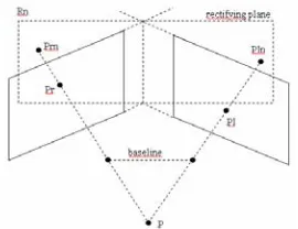
Figure 2. Epipolar geometry
In fig. 2, the triangle lies in the epipolar plane. The lower corners of the triangle (Ol & Or) are the optical centers. The intersections of the triangle’s base with the planes are the epipoles. An epipole represents the image of the center of the opposite camera on the image plane. The dotted lines are the epipolar lines.
The challenge in finding correspondences is the matching process which finds the corresponding features between the left and right images. The matching process can be viewed as a complex optimization problem in which image features are selected, extracted, and matched using a set of constraints that must be satisfied simultaneously.
Figure 3. Ilustration of rectifying Image technique
Corresponding points between two images are found by searching for the point correspondence along an epipolar line. In general, epipolar lines are not aligned with coordinate axis and are not parallel. Such searches are time consuming since we must compare pixels on skew lines in image space. Therefore, we need a method to rectify images [1],[3] to determine transformations of each image plane such that pairs of conjugate epipolar lines become collinear and parallel to one of the image axes (usually the horizontal one).
IV. PREPARE THE SYSTEM
A good Image acquisition system is the first important step to obtain high quality input images. Most imaging sensors (for example CCD and CMOS) are sensitive to the energy of the incoming light but not to its polarization state. Therefore, there is a special setup to get polarization information. It can be obtained by mounting a rotating linear polarizing filter in front of a camera and capturing multiple images with different angles α (with the transmission axis) of the linear polarizer. In this case, the acquisition setup must be able to accommodate the image capture process for
0 2 2 2 1
S S S +
=
ρ
2 1 S arctan
S
extract of polarization information as well as for stereo matches purpose.
A. Image Acquisition
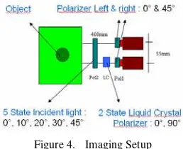
The stereo setup used is shown in fig. 4. Two units of AVT Guppy camera (F-080B monochrome camera) are installed to get stereo images on the baseline. In front of the stereo cameras, we setup an optical device such as polarizer with different alpha values (45° for right camera and 0° for the left camera). In the Left camera, the polarizer was combined with the electric liquid crystal (LC) polarizer to create automated image capture with different alpha values 0° and 90°. We also install another mechanic polarizer rotator to describe the situation of incident light. It will help us to estimate variety of polarized input images.
Figure 4. Imaging Setup
Table 1 presents captured Image scenes to be used to find the best Local Matching for Polarization Images.
TABLE I. CAPTURED IMAGES WITH POLARIZATION SETUP SCENESS Polarizer setting (alpha degree)
No Name Number
of image Pol1
Left Cam
Pol1 Right
Cam
Liquid Crystal left Cam
Pol2 All cam incident
1 Jul15_fix0 (1x2pics) 0 45 0 0
2 Jul15_fix1 (1x2pics) 0 45 90 0
3 Jul15_fix2 (1x2pics) 0 45 0 10
4 Jul15_fix3 (1x2pics) 0 45 90 10
5 Jul15_fix4 (1x2pics) 0 45 0 20
6 Jul15_fix5 (1x2pics) 0 45 90 20
7 Jul15_fix6 (1x2pics) 0 45 0 30
8 Jul15_fix7 (1x2pics) 0 45 90 30
9 Jul15_fix8 (1x2pics) 0 45 0 45
10 Jul15_fix9 (1x2pics) 0 45 90 45
B. Photometric Calibration
Optical devices should be calibrated first to ensure having appropriate alpha values before capturing the images. This step is called photometric calibration. We do this step for every polarizer and for two states of the electric polarizer rotator (0° and 90°). Fig. 5 shows the photometric calibration setup. Images are captured for each value for alpha from 0 to 180 with a predefined step. Computation is based on the Mueller matrix of the linear polarizer and the Stokes vector ((4), (5), (6), (7)). Then, we compare intensity from the original captured images with the predicted intensity from this computation. Ideally, the result is 0. But a difference of one to two pixels can be tolerated, if more it means there is too much noise in the image.
Figure 5. Photometric calibration setup
C. Stereo Calibration and Image Rectification
In order to get the intrinsic and extrinsic stereo system parameters, the stereo system should be calibrated. These parameters are used to rectify images captured by left and right cameras. This simplify corresponding points search on the horizontal lines when both cameras contain the same epipoler line.
Ten pairs of images for the calibration pattern were captured. The system was calibrated using the Matlab camera calibration toolbox from J.Y. Bouguet [8]. We have adapted the method in [1] to rectify the images.
D. Features Extraction
The first step to find correspondences between two input images is to define salient regions to obtain clear matches. Harris corner detector in [6] was used for features extraction. We can calculate the change of intensity by the following equations
(8)
The procedure is as follows:
• Compute the derivatives of the intensity image in the x and y directions for every pixel.
• The squared image derivatives should be smoothed by convolving them with a Gaussian filter.
• Define autocorrelation matrix M for every pixel. M is used to derive a measure of “cornerness”. Rank M = 0, the pixel belongs to a homogeneous region. Rank M = 1, an edge (significant gradients in one directions), and rank M = 2, a corner (significant gradients in both directions).
• Compute Intensity change in a shifting window with eigenvalue analysis E = min (Eigenvalue of M) • Measure of corner response R = det(M)- k·tr(M)2
E. Outliers Rejection and Ground Truth Computation
In order to obtain accurate matching results, we need to make sure that the points found in the second image is in the right position. In this work, for the sake of accuracy of published results, we manually carefully rejected outliers by visual guidance to make sure that the features correspondences between the reference image and the other image satisfy a physically realizable transformation, but in future work, the outliers will be removed automatically.
[
]
2,
( , ) ( , ) ( , ) ( , )
x y
V. MATCHING SCORE METHODS FOR STEREO MATCHING WITH POLARIZATION IMAGING
Brown [2] divided stereo matching methods into two types, local and global methods. In local methods, matching is done by looking for the most similar matches based on local image properties (in predefined neighborhood / window). In global methods, matching relies on iterative schemes that makes disparity assignments, based on the minimization of a global cost function. In this work, we use local methods to analyze every local photometric properties of the neighboring pixels.
A. The Local Matching Algorithms
The matching cost is evaluated based on similarity statistics. The simplest method is to compare pixel intensity values, which is very sensitive to noise and image distortion. More robust matching methods compare windows containing the image neighborhood of processed pixel. Some other methods improve similarity matching by considering three different metrics :
• Correlation, such as NCC (Normalized Cross Correlation), this is a standard statistical method for determining similarity.
• Intensity differences such as SSD (Sum Squared Differences) and it can be normalized as well (Normalized-SSD), and SAD (Sum of Absolute Differences).
• Rank metrics such as rank transform and census transform [14]
In this work, we compared all local matching methods to find the best to be applied on polarized images. Table II shows a full comparison of the following methods.
1) NCC equation [2] :
5) Rank Transform [2]:
(
1 2)
6) Census Transform [2]:
(
1 2)
The polarizer in front of the left camera was set to 0° and 90°, and the one in front of the right camera was set to 45° before capturing images.
To obtain good stereo matching results, we find the match between total intensity image (0°+90°)/2 in the left, and 45° image in the right.
B. Extract Polarization Information
According to Wolff et al. [11], to get state of polarization at least three different intensity images through the polarization filter should be captured. If I0, I45 and I90 are a representation of the image intensity measurements taken at an angle of polarizer of 0°, 45° and 90°, we will have a gray level image from polarized images and compute intensity of polarization, degree of polarization, and angle of polarization based on (1),(2) and (3).
In this work, the polarization state was extracted for each pixel founded by matching algorithm. We use this polarization information as verification to the incident light scene (0 °, 10 °, 20 °, 30°, 45°) which represents various angles of Polarization of incident light. By comparing the angle of Polarization obtained from the calculation at this step, with angle of Polarization conditions in the setup scene of incident light, we will have the certainty that this method is promising.
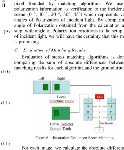
C. Evaluation of Matching Results
Evaluation of stereo matching algorithms is done by comparing the sum of absolute differences between the matching results for each algorithm and the ground truth.
Figure 6. Ilustration Evaluation Score Matching
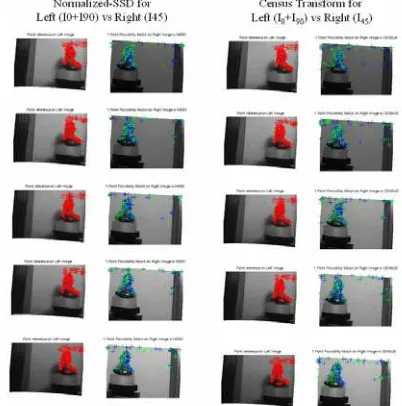
by Harris detector. Fig. 7 illustrates the visualization of matching results of NSSD and Census methods which give best results.
Figure 7. Result Matching stereo by NSSD and Census Transform for Polarized Images
Table II below represents the results of the evaluation of the matching algorithm applied to images with a variety of polarized incident light scene.
TABLE II. EVALUATION RESULT OF 6 MATCHING ALGORITHM FOR EACH SCENES INCIDENT LIGHT (0°,10°,20°,30°,45°)
0° 10° 20° 30° 45°
NSSD 24399.5 23745.5 16375.5 17419 18998
SSD 46337.5 37769.5 27750 31764.5 48746.5
SAD 41758.5 35175.5 25610.5 29084.5 44004
Rank 24192.5 26147 23661.5 22965 23234
Census 25088.5 26134.5 16658 16734.5 19132
NCC 27560.5 27565.5 22463 21024 21543.5
From six local matching methods were compared, we find that the NSSD provides a smaller error than other methods. This means that method can be used to further process associated with stereo matching for the polarized images. The comparison in graphical form can be seen in fig. 8.
Figure 8. Graphics representation for Matching Result 6 Local Algorithm in 5 Incident Light Condition
RESULTS AND CONCLUSION
In this paper we have proposed an imaging setup, which can accommodate polarization based stereo Computation. We also obtain a Normalized SSD method can perform matching with smaller errors than other local method.
In out future work, we will try a various combinations of feature point generate method, such as SIFT and SURF to get more set of pixels that can be compared and use an automatic reject outliers method and some filtering system to make an improvement stereo matching based on polarized images.
ACKNOWLEDGMENT
Thanks to Abd El Rahman Shabayek for valuable discussion and to anonymous referees who made useful comments. This work was supported by grants from Ministry Educational and Cultural, Republic of Indonesia. Optics and all research equipments are courtesy of LE2I Le Creusot, France.
REFERENCES
[1] A. Fusiello, E. Trucco and A. Verri, "A compact algorithm for rectification of stereo pairs", Machine Vision and Applications Springer Journal, Vol12 Number 1:pp 16-22 July, 2000
[2] M. Z. Brown et al, “Advances in Computational Stereo”, IEEE TRANSACTIONS ON PATTERN ANALYSIS AND MACHINE INTELLIGENCE, VOL. 25, NO. 8:pp 993-1008, 2003.
[3] C. Loop, Z. Zhang, "Computing rectifying homographies for stereo vision", Proc. IEEE Computer Vision and Pattern Recognition, Vol.1 :pp 125-131, Juni 1999.
[4] L.D. Stefano et al, “A fast area-based stereo matching algorithm”, Elsevier Image and Vision Computing journal, journal 22:pp 983-1005, 2004.
[5] D. Goldstein, “Polarized Light”, Second Edition, CRC Press, ISBN-13: 9780824740535, 2003.
[6] Harris and M. Stephens. “A combined corner and edge detector”, Fourth Alvey Vision Conference, Manchester, UK, pp. 147-151, 1988.
[7] Humenberger, Martin, Evaluation of Stereo Matching Systems for Real World Applications Using Structured Light for Ground Truth Estimation, MVA2007 IAPR Conference on Machine Vision Applications, May 16-18, 2007, Tokyo, JAPAN, 2007.
[8] J.Bouguet. Matlab camera calibration toolbox, Website Caltech.Edu http://www.vision.caltech.edu/bouguetj/calib doc/index.html, July, 2008.
[9] L.B. Wolff, “Polarization Bases Material Classification from specular reflection”, IEEE transactions on Pattern Analysis and Machine Intelligence, Vol 12:pp. 1059-1071, 1990.
[10] L.B. Wolff and A. Andreou, “Polarization Camera Sensor” Image and Vision Computing Journal, Vol 13 Number 16: pp. 497-510 , 1995. [11] L.B. Wolff, “Polarization Vision : a new sensory approach to Image
Understanding”, Image and Vision Computing Elsevier Journal, Vol 15:pp. 81-93, 1997.
[12] L.B. Wolff, “Liquid Crystal Polarization Camera”, IEEE transactions on Robotics and Automation, Vol 13:pp. 195-203, April 1997. [13] R. Hartley and A. Zisserman, Multiple View Geometry in Computer
Vision. Cambridge: UK, Cambridge Univ. Press, 2000.
[14] R. Zabih and J. Woodfill. “Non-parametric local transforms for computing visual correspondence”, Proc. of the Third European Conference, vol 2:pp. 151-158, 1994.
0 10000 20000 30000 40000 50000 60000