11 (2000) 473 – 489
Engines of growth in the US economy
Thijs ten Raa
a,*, Edward N. Wolff
baDepartment of Economics,Tilburg Uni6ersity,Box90153,NL-5000LE Tilburg,Netherlands bDepartment of Economics,New York Uni6ersity,269Mercer Street,New York,NY10003, USA
Received 1 November 1999; received in revised form 1 July 2000; accepted 29 August 2000
Abstract
There is good reason to believe that R&D influences on TFP growth in other sectors are indirect. For R&D to spill over, it must first be successful in the home sector. Indeed, observed spillovers conform better to TFP growth than to R&D in the upstream sectors. Sectoral TFP growth rates are thus inter-related. Solving the intersectoral TFP equation resolves overall TFP growth into sources of growth. The solution essentially eliminates the spillovers and amounts to a novel decomposition of TFP growth. The top 10 sectors are designated ‘engines of growth’ led by computers and office machinery. The results are contrasted with the standard, Domar decomposition of TFP growth. © 2000 Elsevier Science B.V. All rights reserved.
JEL classification:O30; O41; O51; L86; D57
Keywords:Input – output; Sources of growth; Spillovers
www.elsevier.nl/locate/strueco
1. Introduction
Spillovers of technical change are known to drive a wedge between private and social rates of return to research and development (R&D). What is less known, is that spillovers render total factor productivity (TFP) growth in some sectors more critical than in others. While it is true by growth accounting that we may decompose macro TFP growth into sectoral components and thus identify the progressive sectors, this procedure amounts to a neutral addition of sectoral TFP growth rates. The contribution of a sector’s TFP growth is determined by the value
* Corresponding author. Tel.: +31-13-4662365; fax:+31-13-4663280.
share of the sector in the total economy, without one sector being more critical than another. The picture changes slightly, but no more than that, when we regress TFP growth on R&D in a panel of sectors. Here, too, R&D may turn out to be more influential when spent in some sectors, but the mechanics of growth accounting remain the same, and TFP growth is not more critical in those sectors.
The story takes a twist when R&D influences TFP growth in other sectors not directly, but indirectly, that is, only after it has been proven successful in the sector where it has been spent. If this is the case, then spillovers inter-relate sectoral TFP growth rates and we may expect multiplier effects. The multipliers will depend on the spillover relationships, and these need not be equal to the structure of the material balances in the economy. Hence, TFP multiplier effects are not given by the standard multiplier matrix, the Leontief inverse.
There is good reason to believe that R&D influences on TFP growth in other sectors are indirect. For R&D to spill over, it must first be successful in the home sector. Indeed, observed spillovers conform better to TFP growth than to R&D in the upstream sectors, as noted in Wolff (1997). Hence it is of utmost interest to determine which sectors transmit technical change more strongly. These sectors are the engines of growth. Engines of growth need not feature high R&D, but once they move in terms of own TFP growth, they push the entire economy.
The interdependence of sectoral TFP growth rates is given by a system of equations that account for the spillover effects. In this paper we solve the spillover equations for TFP growth rates. The reduced form of the TFP growth rates shows their dependence on sectoral R&D expenditures, and the coefficients measure total returns to R&D, including the spillover effects. Observed sectoral TFP growth rates are thus ascribed to sources of growth.
Direct sectoral decompositions of TFP growth impute little to automation. As Bob Solow noticed: ‘‘You can see the Computer Age everywhere but in the productivity statistics.’’ Our solution of the spillover structure will reveal computers as a primary engine of growth.
In the next section we review some of the literature. In Section 3 we present the general equilibrium analysis of TFP spillovers. We decompose TFP growth not only by sectoral TFP growth in an accounting fashion, but also by sources of growth. We do so by solving the TFP equation for its multiplier structure. Engines of growth are defined formally. Then, in Section 4, we describe the data set we use. Results for the US economy are presented in Section 5 and Section 6 concludes.
2. Review of the literature
material and capital purchases made by one industry from supplying industries. Scherer (1982), relying on Federal Trade Commission line of business data, used product (in contradistinction to process) R&D, aimed at improving output quality, as a measure of R&D spillovers.
Another approach is to measure the ‘technological closeness’ between industries, even if they are not directly connected by interindustry flows. For example, if two industries use similar processes (even though their products are very different or they are not directly connected by interindustry flows), one industry may benefit from new discoveries by the other industry. Such an approach is found in Jaffe (1986), who used patent data to measure technological closeness between industries. The patent approach to spillovers has been continued by Evenson and Johnson (1997), Kortum and Putnam (1997), Verspagen (1997) and Verspagen and Los (2000).
Bernstein and Nadiri (1989) use as a measure of intra-industry R&D spillovers total R&D at the two-digit SIC level and apply this measure to individual firm data within the industry. Mairesse and Mohnen (1990) report similar results by compar-ing R&D coefficients based on firm R&D with those based on industry R&D. If there are intra-industry externality effects of firm R&D, then the coefficients of industry R&D should be higher than those of firm R&D. However, their results do not show that this is consistently the case. (Also see Mohnen, 1992a and Griliches, 1992 for reviews of the literature.)
A different approach was followed by Wolff and Nadiri (1993), who used as their measure of embodied technical change a weighted average of the TFP growth of supplying industries, where the weights are given by the input – output coefficients of an industry. This formulation assumed that the knowledge gained from a supplying industry is in direct proportion to the importance of that industry in a sector’s input structure. Wolff (1997) updated these earlier results using US input – output data for the period 1958 to 1987, and found strong evidence that industry TFP growth is significantly related to the TFP performance of supplying sectors, with an elasticity of almost 60 percent. The results also indicated that direct productivity spillovers were more important than spillovers from the R&D per-formed by suppliers.
The later studies generally tend to be more positive. Both Siegel and Griliches (1992) and Steindel (1992) estimated a positive and significant relationship between computer investment and industry-level productivity growth. Lau and Tokutso (1992) estimated that about half of real output growth in the United States could be attributed directly or indirectly to IT investment. Oliner and Sichel (1994) reported a significant contribution of computers to aggregate US output growth. Lichtenberg (1995) estimated firm-level production functions and found an excess return to IT equipment and labor. Siegel (1997), using detailed industry-level manufacturing data for the US, found that computers are an important source of quality change and that, once correcting output measures for quality change, computerization had a significant positive effect on productivity growth. Brynjolfs-son and Hitt (1996, 1998) found a positive correlation between firm-level productiv-ity growth and IT investment over the 1987 – 1994 time period, particularly when accompanied by organization changes. Lehr and Lichtenberg (1998) used data for US federal government agencies over the 1987 – 1992 period and found a significant positive relation between productivity growth and computer intensity. Lehr and Lichtenberg (1999) investigated firm-level data among service industries over the 1977 – 1993 period and also reported evidence that computers, particularly personal computers, contributed positively and significantly to productivity growth.
Two studies looked, in particular, at R&D spillovers embodied in IT investment. Bernstein (1995) found a positive and highly significant influence of R&D linked (both embodied and disembodied) in communication equipment on the TFP growth of industries using this equipment. van Meijl (1995) also estimated a positive and significant effect of R&D embodied in IT investment in general on TFP growth in other sectors. Both, moreover, found that the spillover effect was increasing rapidly over time.
Technological sources of growth have been documented by economic historians (Landes, 1969) and modeled by Amable (1993) and many others, but it is only fairly recently that attempts have been made to pinpoint sources of growth in a micro-economic or at least multi-sectoral framework. The term ‘engines of growth’ has been coined by Bresnahan and Trajtenberg (1995). Their central notion is that a handful of ‘general purpose technologies’ bring about and foster generalized productivity gains throughout the economy. The productivity of R&D in a down-stream sector increases as a consequence of innovation in the general purpose technology. Bresnahan and Trajtenberg (1995) proceed to construct a partial equilibrium model of an upstream sector and a downstream sector, and then examine the welfare consequences of a simple one-step innovation game. Our model, however, is general equilibrium; the interaction between sectors is circular and there is no presumed engine of growth. While the terminology of Bresnahan and Trajtenberg (1995) is suggestive and useful indeed, it remains to identify the engines of growth given the body of input – output data that represent the structure of a national economy.
with workers recouping their training costs. The invention of the new technology is exogenous and its spread is determined by the mechanics of utility maximization in a dynamic economy with a single output. These authors take the source of the new technology for granted and examine its propagation and productivity effects. We start at the other end, the sectoral productivity growth rates, and try to trace back the sources of growth, in terms of sectoral R&D activities. We do so by solving the spillover structure for its reduced form. Unlike Caselli (1999) and Helpman and Rangel (1999), we were not motivated by the information technology revolution, but by the sheer theoretical challenge to pinpoint sources of growth in a general equilibrium input – output framework.
3. Productivity analysis of spillovers
Our point of departure is the Solow residual definition of total factor productiv-ity (TFP) growth,P:
P=(pdy−wdL−rdK)/(py) (1) Herey is the final demand vector,Lis labor input,Kis capital input,wandrtheir respective prices, and p is the row vector of production prices, reflecting zero profits:
p(I−A)=6=wl+rk (2)
whereAis the matrix of the intermediate input coefficients and 6,l and kare the raw vectors of value-added, labor and capital coefficients. As Solow (1957) showed, the zero profit condition is needed to let the residual measure technical change. More precisely, the numerator of residual Eq. (1) becomes
pd[(I−A)x]−wd(lx)−rd(kx)
=(−pdA−wdl−rdk)x+[p(I−A)−wl−rk]dx (3)
where the last term vanishes only if we use the production prices of Eq. (2). Then TFP growth defined by Eq. (1) reduces to
P= −(pdA+wdl+rdk)x/(py)=ppˆx/(py) (4) where
= −(pdA+wdl+rdk)pˆ−1
(5)
is the row vector of sectoral TFP growth rates andpˆx/(py) is the column vector of Domar weights.
growth of other sectors it must first be successful in the home sector, and this success is measured by its effect in terms of TFP growth. Second, we wish to endogenize the general equilibrium transmission of spillovers. Instead of putting in total input coefficients (the standard Leontief inverse) into the equation (as do Sakurai et al., 1997), we want to obtain them by solving the equation. Third, TFP growth based spillovers yield the best fit, according to Wolff (1997).
We distinguish four sources of sectoral TFP growth, pj, an autonomous source,
a, R&D in sectorj per dollar of gross output, denoted by
rj=RDj/(pjxj) (6)
a direct productivity spilloverS(piaij/pj)pi, and a capital embodied spilloverS(pibij/
pj)pi, wherebijis the investment coefficient of capital goodiin sector j, per unit of
output. We first regress sectoral TFP growth as follows (denoting the vector with all entries equal to one by e):
p=aeT+b
1r+b2ppˆApˆ−1+b3ppˆBpˆ−1+o (7) wherea,b1, and b2 are coefficients ando is a stochastic error term (Wolff, 1997). The weights of the sources are assumed to be constant across sectors. If we denote the spillover matrix by
C=b2pˆApˆ−1+b3pˆBpˆ−1 (8)
then Eq. (7) reads, ignoring the error term
p=aeT
+b1r+pC (9)
To interpret the regression coefficient as a return to R&D (Mohnen, 1992b), we relate TFP growth to R&D both directly and indirectly, that is through the spillovers. The direct effect is obtained by substituting Eqs. (6) and (9) into Eq. (4):
P = [aeT+b
1RD(pˆxˆ)−1+pC]pˆx/(py)
= aDR+b1RDe/(py)+pCpˆx/(py)
(10)
whereRDis the row vector with elementsRDjgiven by Eq. (6) andDR=(px)/(py),
the Domar ratio, and RDe is the total R&D expediture, summed over sectors. There are two, equivalent interpretations ofb1. First, sinceP is a growth rate, b1 measures therate of return to R&D intensity, where the latter is taken with respect to the value of net output or GDP. Second, since the denominator in the definitions ofP, see Eq. (1), is alsopy, the equality of the numerators in Eq. (10) reveals that b1measures thereturn to R&D, in terms of output value per dollar expenditure.b1 measures the direct rate of return to R&D intensity or, equivalently, the direct return to R&D. Now notice that the last term of Eq. (10), the intermediate inputs and embodied TFP growth rates, features the row vector of sectoral TFP growth rates,p, and, therefore, reinforces the effect of R&D on productivity through the spillovers.
M=(I−C)−1
=I+C+C2
+··· (11)
Sakurai et al. (1997) model indirect spillover effects by putting the standard Leontief inverse directly into the TFP regression equation. We, however, model the direct spillovers and determine the indirect ones by general equilibrium analysis of the transmission mechanism, solving Eq. (9) using Eq. (11):
p=(aeT
+b1r)M (12)
The direct rate of return to R&D was based on b1r. The total rate of return is obtained by inflation through multiplier matrixM in Eq. (11). Here I reproduces the direct rate of return,C, specified in Eq. (8), produces the direct spillover effect, and C2+··· the indirect spillover effects. The TFP growth expression in Eq. (4) becomes
P=ppˆx/(py)=(aeT
+b1r)Mpˆx/(py) (13)
Eq. (13) reduces TFP growth not only to sectoral TFP growth rates, but also to autonomous TFP growth and sectoral R&D expenditures. The middle expression in Eq. (13) is the usual Domar decomposition of TFP growth, Eq. (4). The right-hand side of Eq. (13) is an alternative, novel decomposition:
P=[(a+b1r1)%
j
m1jpjxj+···+(a+b1rn)% j
mnjpjxj]/(py) (14)
Again, there are two, equivalent measures for the productivity effect of R&D. The
total rate of return to R&D intensityri amounts to b1(Sjmijpjxj)/(py). Here b1 is deflated by multipliers mij because of the spillover effects and also by gross/net
output ratios as the sectoral R&D intensities ri are defined as the R&D/gross
output ratios (which are small because of the denominators).
Once more, the second interpretation is derived from the observation that either side of Eq. (14) haspyas denominator. Hence thetotal return to R&D, in terms of output value per dollar expenditure in sector i, amounts to b1(Sjmijpjxj)/(pixi)
using Eq. (6). Notice that the direct return to R&D, b1, is inflated by the factor (Sjmijpjxj)/(pixi) because of the spillover effects stemming from sector i. Notice
also that some sectors have stronger spillover effects than others, as determined by the rows of the multiplier matrix. The factors (Sjmijpjxj)/(pixi) reinforce the
returns to R&D and are, therefore, spillo6er multipliers. Spillover multipliers are related to the standard forward multipliers of input – output analysis (the row totals of the standard Leontief inverse), but there are two differences. First, spillover multipliers are based on the Leontief inverse of spillover matrix C rather than technology matrix A. Second, spillover multipliers are not straight row sums, but weighted by output value ratios (pjxj)/(pixi). We shall compare spillover multipliers
to standard forward multipliers for the US economy. Spillover multipliers account for the ratio of the total to the direct return to R&D and, therefore, measure the external effect of sectoral R&D.
Eq. (14) shows that the contribution of a sector to TFP growth can be high for two reasons. First, the intensity of R&D can be high. Second, the spillover factor
sources of growth,a+b1r1for sector 1 toa+b1rnfor sectorn, aggregated by the
(forward) linkages, Sjm1jpjxj for sector 1 to Sjmnjpjxj for sector n. Whereas the
first decomposition, Eq. (4), is a TFP growth accounting identity, the second decomposition, Eq. (14), imputes TFP growth to sources of growth taking into account the general equilibrium spillover effects. Sectors that pick up much TFP growth in decomposition Eq. (14) are theengines of growth. The greatest engine of growth is the sector, sayi, with the greatest value of (a+b1ri)Sjmijpjxj. Whereas
sectors with high TFP growth can be identified by direct growth accounting in the sense of Domar, engines of growth reveal themselves only after solving the intersectoral TFP growth rates equation for spillover effects to its reduced form, Eq. (13).
4. Data sources
The basic data are 85-sector US input – output tables for years 1958, 1967, 1977, and 1987.1 Labor coefficients were obtained from Bureau of Labor Statistics’ Historical Output and Employment Data Series (obtained on computer diskette).2 Capital stock by input – output industry for 1967 and 1977 was calculated directly from the net stocks of plant and equipment by input – output industry provided on computer tape by the US Bureau of Industry Economics (the BIE Capital Stocks Data Base as of January 31, 1983). These series ran through 1981 for manufactur-ing industries and through 1980 for the other sectors. They were updated to 1987 on the basis of the growth rate of constant dollar net stock of fixed capital between 1980 (or 1981) and 1987 calculated from the National Income and Product Accounts (NIPA).3
Sectoral price indices were calculated from the Bureau of Labor Statistics’ Historical Output Data Series (obtained on computer diskette) on the basis of the current and constant dollar series.4
1Details on the construction of the input – output tables can be found in the following publications:
1967, US Interindustry Economics Division (1974); US Interindustry Economics Division (1984); and 1987, Lawson and Teske (1994). We aggregate sectors 1 – 4, 5&6, 9&10, 11&12, 20&21, 22&23, 33&34, 44&45 and delete 74 and 80 – 85. Thus we partition the US economy in 68 sectors.
2Data on hours worked by sector, though the preferable measure of labor input to employment, are
not available by sector and year and therefore could not be incorporated.
3The source is Musgrave (1992). Since there are fewer industries in the NIPA breakdown than in the
input – output data, we applied the same percentage growth rate across all input – output industries falling within a given NIPA classification. Data on government-owned capital stock for all years were obtained from Musgrave (1992).
4In addition, the deflator for transferred imports was calculated from the NIPA import deflator, that
Five sectors — research and development, business travel and office supplies, scrap and used goods, and inventory valuation adjustment — appeared in some years, but not in others (the earlier years for the first three sectors and the later years for the last two sectors). In order to make the accounting framework consistent over the four years of analysis, we eliminated these sectors from both gross and final output. This was accomplished by distributing the inputs used by these sectors proportional to either the endogenous sectors which purchased the output of these five sectors or the final output.5
Data on the ratio of R&D expenditures to GDP were obtained from the National Science Foundation,Research and De6elopment in Industry, various years, for 32 manufacturing industries covering the period 1958 to 1987. We were able to allocate these figures to 48 manufacturing industries in the input – output data.6
5. Results
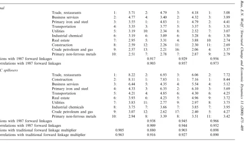
Table 1, upper panel, shows the standard forward multipliers for the 68 indus-tries in each of the four years. In 1987, not surprisingly, wholesale and retail trade is the sector with the highest forward linkage, since, by construction, it supplies almost all industries in the economy. The second most important supplier is the business service sector, followed by primary iron and steel, transportation, utilities, and industrial chemicals. On the bottom of the list are the consumer-oriented sectors, including tobacco products, ordinance (that is, armaments), household appliances, and footwear and leather products. Cross-industry correlations in forward linkages are very high, though they tend to attenuate over time. The correlation coefficient between the 1987 and 1977 forward linkages is 0.96, com-pared with a correlation of 0.92 between the 1958 and 1987 linkages; the respective rank correlations are 0.97, 0.96, and 0.90.
We next compute the new forward linkages based on matrix C. Results on forward linkage multipliers based on Eq. (7) witha=0.003,b1=0.106,b2=1.101 and b3=0.753 (following Wolff, 1997) are shown in Table 1, lower panel. There are now some interesting differences between these new multipliers and the stan-dard forward linkage multipliers. On the basis of the 1987 multipliers, the trade sector ranks first and the construction sector ranks second, which is not unexpected since new investment is incorporated in the multiplier calculation. Business services
5The allocation of the scrap sector was handeled differently in the make-use framework of the 1967,
1977 and 1987 tables. See ten Raa and Wolff (1991) for details.
6This was calculated in two steps. First Company R&D from the Federal Trade Commission Line of
T
Ranks and values of forward linkage multipliers based onpˆApˆ−1(traditional) and matrixCspillovers, 1958–1987, with sectors ranked by 1987 multipliers
(top 10 only)
Transportation 4: 3.35 3: 5: 3.37 5: 3.31
55
8: 2.52 7: 3.07
58 Utilities 5: 3.19 10: 2.34
6: 3.28 6: 3.30
3.09
19 Industrial chemical 6: 3.19 6:
4: 3.88 10: 2.74
61 Real estate 7: 2.95 5: 3.31
11: 2.30 11: 2.69 2.26
6 Construction 8: 2.59 12:
4 Crude petroleum and gas 9: 2.57 13: 2.21 16: 2.06 4: 3.37
7: 2.87 9: 2.79
2.78 7:
29 Primary non-ferrous metals 10: 2.51
Correlations with 1987 forward linkages 0.917 0.929 0.956
0.957 0.973
0.903 Rank correlations with 1987 forward linkages
Matrix C spillo6ers
6 Construction 2: 8.11 1: 7.83 8.44
4: 5.54 4: 5.12
4.35
63 Business services 3: 6.44 5:
Primary iron and steel 4: 4.33 6.35 2: 6.10 3: 5.69
28 3:
58 Utilities 7: 3.83 11: 2.77 2.97 8: 3.75
7: 3.85 7: 3.95
3.66
19 Industrial chemicals 8: 3.75 7:
17: 2.40 5: 4.27
4 Crude petroleum and gas 9: 3.07 12: 2.62
8: 3.51 11: 3.42 3.39
29 Primary non-ferrous metals 10: 2.94 8:
0.945 0.966
Correlations with 1987 forward linkages 0.938
0.909 0.952
Rank correlations with 1987 forward linkages 0.944
0.905 0.880 0.903
Correlations with traditional forward linkage multiplier 0.898
now rank third, followed by primary iron and steel and transportation. The correlation coefficients between the new forward linkage multipliers and the stan-dard forward linkage multipliers are now around 0.9, and the rank correlations range from 0.89 to 0.96. Cross-industry correlations in these new forward link-ages are high and increase over time. The correlation coefficient between the 1987 and 1958 forward linkages is 0.94, that between the 1987 and 1967 multi-pliers is 0.95; and that between the 1987 and 1977 multimulti-pliers is 0.97; the corresponding rank correlations are 0.91, 0.94, and 0.95.
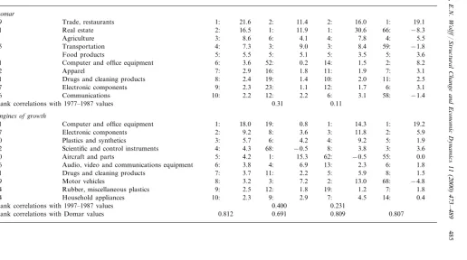
We next look at the major spillover sectors over the 1958 – 1987 period. These are defined as sectors i with high spillover terms pi(ci1 … cin) which reflect both
the strength of their forward linkages and their TFP growth. These sectors, shown in Table 2, are the ones which contributed most to the overall TFP growth of the economy. Over the whole 1957 – 1987 period, the most important source of overall growth was the trade sector, reflecting its very high forward linkage value. The second most important sector was computer and office equip-ment, a reflection of its very high TPF growth. Indeed, in the 1977 – 1987 period, it made by far the greatest contribution to embodied TFP growth. The third most important sector over the 1958 – 1987 period was electronic components, followed by transportation and plastics and synthetics. At the bottom of the list are the low (actually negative) TFP growth sectors, including crude petroleum and gas, finance and insurance, business services, radio and TV broadcasting, and metallic mining.
It is also of interest that there is very little correlation over time in the rank order (or values) of sectors in terms of pC. The correlation coefficient between the 1958 – 1967 and the 1977 – 1987 values is 0.27 and the rank correlation is 0.22; the corresponding figures between the 1967 – 1977 and 1977 – 1987 values are
−0.03 and 0.12. This is a reflection of the fact that sectoral TFP growth is very variable over time.
T
Embodied total factor productivity growth rates, based onpi(ci1 … cin) in Eq. (9), 1958–1987, with sectors ranked by 1958–1987 values (top 10 only,
figures in percent per annum)
41 Computer and office equipment 2: 6.4 50: 0.7 14.5
5: 4.7 3: 7.6
4.0 9:
47 Electronic components 3: 5.7
2: 7.6 58: −1.9
55 Transportation 4: 5.1 1: 10.0
4: 5.3 6: 4.8
4.9
20 Plastics and synthetics 5: 5.1 6:
3: 6.5 1: 12.9 62: −2.9
53 Ophthalmic and photographic equipment 8: 2.5 18: 3.1
23: 1.4 12: 2.9
3.1
10 Fabrics, yarn and thread mills 9: 2.4 17:
14: 3.2 43: 0.3 9: 3.7
10:
24 Rubber, miscellaneous plastics 2.4
Correlations with 1977–1987 values 0.274 −0.028
485
Percentage decomposition of overall TFP growth by sector, based on Eq. (4) (Domar) and Eq. (14) (sources of growth), with sectors ranked by 1958–1987 values (top 10 only, figures in percent per annum, with denominator the sum of positive elements only)
1967–1977 1977–1987
41 Computer and office equipment 6:
1.8
Apparel 7: 2.9 16: 11: 1.9 7: 3.1
12
10: 2.0 11: 2.5
21 Drugs and cleaning products 8: 2.4 19: 1.4
12: 1.7 6: 3.1
1.1 Electronic components
47 9: 2.3 23:
2.2
Communications 10: 2.2 12: 6: 3.1 58: −1.4
56
Computer and office equipment 18.0 19: 0.8 41
3: 11.8 2:
47 Electronic components 2: 9.2 8: 3.6 5.9
4: 9.2 5: 1.9
4.2
20 Plastics and synthetics 3: 5.7 6:
68: −0.5 8: 3.8 3: 3.6
4:
52 Scientific and control instruments 4.3
62: −0.5 55: 0.0 15.3
Aircraft and parts
50 5: 4.2 1:
6.9
Audio, video and communications equipment 6: 3.8 4: 13: 2.3 6: 1.8 46
11: 2.2 5: 5.9 8: 1.5
21 Drugs and cleaning products 7: 3.7
2: 13.0 68: −4.8 7.2
3.2 3:
49 Motor vehicles 8:
1.8
Rubber, miscellaneous plastics 9: 2.5 12: 19: 1.2 7: 1.8
24
7:
44 Household appliances 10: 2.3 9: 2.9 4.5 14: 0.4
Rank correlations with 1997–1987 values 0.400 0.231
0.812 0.691 0.809 0.807
sector was electronic components, which accounted for 14% of the positive con-tributions of overall TFP growth over the full 1958 – 1987 period and for 6% in 1977 – 1987. Plastics and synthetics ranked third over the three decades, followed by scientific and control equipment and then aircraft and parts. Together, the top five industries were responsible for 41% of the positive contributions of overall TFP growth over the full 1958 – 1987 period and for 31% in 1977 – 1987. It is also notable that the top 10 industries are all manufacturing industries.
There is very little correlation over time in the rank order of sectors in terms of their contribution to overall TFP growth. The rank correlations between the 1958 – 1967 and the 1977 – 1987 values is 0.40 and that between the 1967 – 1977 and 1977 – 1987 values is 0.23. This again is a reflection of the fact that sectoral TFP growth in the US economy can change radically over time. It also suggests that the engines of growth in the US economy can change radically over time. In the real estate sector, for example, annual TFP growth, after rising from 1.42% in the 1958 – 1967 period to 2.97% in 1967 – 1977, plummeted to −0.76% in 1977 – 1987. This, together with its linkages to other industries in the econ-omy, also accounts for its very low ranking in the 1977 – 1987 period.
A comparison with the standard decomposition of overall TFP growth based on Domar factors (Eq. (4)) is also instructive (see the top panel of Table 3). Here, the top four industries, in rank order, over the 1958 – 1987 period are wholesale and retail trade (including restaurants), real estate, agriculture, and transportation. Computers and office equipment rank only sixth, compared with their top rank on the basis of matrix C. Like the engines of growth, there is a positive but low correlation in rank order of these industries over time, because of the high variability of TFP growth between periods. However, overall, the Domar rankings are similar to those based on matrix C, with rank correlations of 0.8 or so for most periods and for the entire 1958 – 1987 period. This result reflects the fact that industry-level TFP growth is the main determinant of the contribution of an industry to overall TFP growth.
6. Conclusion
Acknowledgements
We are grateful to the C.V. Starr Center for Applied Economics at New York University and to CentER at Tilburg University for visitorships. A referee provided very useful suggestions.
References
Amable, B., 1993. Catch-up and convergence: a model of cumulative growth. International Review of Applied Economics 7 (1), 1 – 25.
Bailey, M., Gordon, R., 1988. The productivity slowdown, measurement issues, and the explosion in computer power. Brookings Papers on Economic Activity 2, 347 – 432.
Berndt, E.R., Morrison, C.J., 1995. High-tech capital formation and economic performance in US manufacturing industries. Journal of Econometrics 69, 9 – 43.
Bernstein, J.I., Nadiri, M.I., 1989. Research and development and intra-industry spillovers: an empirical application of dynamic duality. Review of Economic Studies 56, 249 – 269.
Bernstein, J.I., 1995. The Canadian communication equipment industry as a source of R&D spillovers and productivity growth. Paper presented at the Conference of Implications of Knowledge-Based Growth for Micro-Economic Policies, March 30 – 31, Ottawa, Ontario, Canada.
Bresnahan, T., 1986. Measuring the spillovers from technical advance: mainframe computers in financial services. American Economic Review 74 (4), 743 – 755.
Bresnahan, T.F., Trajtenberg, M., 1995. General purpose technologies engines of growth. Journal of Econometrics 65 (1), 83 – 108.
Brown, M., Conrad, A., 1967. The influence of research on CES production relations. In: Brown, M. (Ed.), The Theory and Empirical Analysis of Production. In: Studies in Income and Wealth, vol. Vol. 3. Columbia University Press for the NBER, New York.
Brynjolfsson, E., Hitt, L., 1996. Computers and productivity growth: firm-level evidence. Mimeo, MIT Sloan School, July.
Brynjolfsson, E., Hitt, L., 1998. Information technology and organizational design: evidence from micro data. Mimeo, MIT Sloan School, January.
Caselli, F., 1999. Technological revolutions. American Economic Review 89 (1), 78 – 102.
Evenson, R.E., Johnson, D., 1997. Introduction: invention input – output analysis. Economic Systems Research 9 (2), 149 – 160.
Goto, A., Suzuki, K., 1989. R&D capital, rate of return on R&D investment and spillover of R&D in Japanese manufacturing industries. Review of Economics and Statistics 71 (4), 555 – 564.
Griliches, Z., 1979. Issues in assessing the contribution of research and development to productivity growth. Bell Journal of Economics 10, 92 – 116.
Griliches, Z., 1992. The search for R&D spillovers. Scandinavian Journal of Economics 94, 29 – 47. Helpman, E., Rangel, A., 1999. Adjusting to a new technology: experience and training. Journal of
Economic Growth 4(4), 359 – 383.
Jaffe, A.B., 1986. Technology opportunity and spillovers of R&D: evidence from firms’ patents, profits, and market value. American Economic Review 76, 984 – 1001.
Kortum, S., Putnam, J., 1997. Assigning patents to industries: tests of the Yale Technology Concor-dance. Economic Systems Research 9 (2), 161 – 176.
Landes, D., 1969. The Unbound Prometheus. Cambridge University Press, Cambridge.
Lau, L., Tokutso, I., 1992. The impact of computer technology on the aggregate productivity of the United States: an indirect approach. Mimeo, Stanford University Department of Economics. Lawson, A.M., Teske, D.A., 1994. Benchmark input – output accounts for the US economy, 1987.
Survey of Current Business 74, 73 – 115.
Lehr, W., Lichtenberg, F., 1999. Information technology and its impact on productivity: firm-level evidence from government and private data sources, 1977 – 1993. Canadian Journal of Economics 32 (2), 335 – 362.
Lichtenberg, F.R., 1995. The output contribution of computer equipment and personnel: a firm level analysis. Economics of Innovation and New Technology 3 (4), 201 – 217.
Loveman, G.W., 1988. An assessment of the productivity impact of information technologies. In: Management in the 1990s. MIT Press, Cambridge, MA.
Mairesse, J., Mohnen, P., 1990. Recherche-developpment et productivite: un sorvoi de la litterature econometrique. Economie et Statistique 237/238, 99 – 108.
Mohnen, P., 1992a. New technology and interindustry spillovers. Science/Technology/Industry Review 7, 131 – 147.
Mohnen, P., 1992b. The relationship between R&D and productivity growth in Canada and other major industrialized countries, Canada Communications Group, Ottawa, Canada.
Musgrave, J.C., 1992. Fixed reproducible tangible wealth in the United States, revised estimates. Survey of Current Business 72, 106 – 137.
National Science Foundation, Research and Development in Industry, Government Printing Office, Washington, DC, various years.
Oliner, S., Sichel, D., 1994. Computers and output growth revisited: how big is the puzzle? Brookings Papers on Economic Activity 2.
Parsons, D.J., Gotlieb, C.C., Denny, M., 1993. Productivity and computers in Canadian banking. Journal of Productivity Analysis 4, 91 – 110.
Sakurai, N., Papaconstantinou, G., Ioannides, E., 1997. Impact of R&D and technology diffusion on productivity growth: empirical evidence for 10 OECD countries. Economic Systems Research 9 (1), 81 – 109.
Scherer, F.M., 1982. Interindustry technology flows and productivity growth. Review of Economics and Statistics 64, 627 – 634.
Siegel, D., Griliches, Z., 1992. Purchased services, outsourcing, computers, and productivity in manu-facturing. In: Griliches, Z. (Ed.), Output Measurement in the Service Sector. University of Chicago Press, Chicago.
Siegel, D., 1997. The impact of computers on manufacturing productivity growth: a multiple-indica-tors, multiple-causes approach. Review of Economics and Statistics, 68 – 78.
Solow, R.M., 1957. Technical change and the aggregate production function. Review of Economics and Statistics 39 (3), 312 – 320.
Steindel, C., 1992. Manufacturing productivity and high-tech investment. Federal Reserve Bank of New York Quarterly Review 17, 39 – 47.
ten Raa, T., Wolff, E.N., 1991. Secondary products and the measurement of productivity growth. Regional Science and Urban Economics 21 (4), 581 – 615.
Terleckyj, N.W., 1974. Effects of R&D on the productivity growth of industries: an exploratory study, National Planning Association, Washington, DC.
Terleckyj, N.W., 1980. Direct and indirect effects of industrial research and development on the productivity growth of industries. In: Kendrick, J.W., Vaccara, B. (Eds.), New Developments in Productivity Measurement. National Bureau of Economic Research, New York.
US Council of Economic Advisers, 1992. Economic Report of the President, US Government Print-ing Office, WashPrint-ington, DC.
US Interindustry Economics Division, 1974. The input – output structure of the US economy, 1967. Survey of Current Business 54, 24 – 56.
US Interindustry Economics Division, 1984. The input – output structure of the US economy, 1977. Survey of Current Business 64, 42 – 84.
van Meijl, H., 1995. Endogenous technological change: the influence of information technology, theoretical considerations and empirical results. Ph.D. Thesis, Maastricht.
Verspagen, B., Los, B., 2000. R&D spillovers and productivity: evidence from US manufacturing microdata. Empirical Economics 25 (1), 127 – 148.
Wolff, E.N., Nadiri, M.I., 1993. Spillover effects, linkage structure, and research and development. Structural Change and Economic Dynamics 4, 315 – 331.
Wolff, E.N., 1997. Spillovers, linkages, and technical change. Economic Systems Research 9 (1), 9 – 23.