Existence and Construction of Vessiot Connections
⋆Dirk FESSER † and Werner M. SEILER ‡
† IWR, Universit¨at Heidelberg, INF 368, 69120 Heidelberg, Germany
E-mail: [email protected]
‡ AG “Computational Mathematics”, Universit¨at Kassel, 34132 Kassel, Germany
E-mail: [email protected]
URL: http://www.mathematik.uni-kassel.de/∼seiler/
Received May 05, 2009, in final form September 14, 2009; Published online September 25, 2009
doi:10.3842/SIGMA.2009.092
Abstract. A rigorous formulation of Vessiot’s vector field approach to the analysis of ge-neral systems of partial differential equations is provided. It is shown that this approach is equivalent to the formal theory of differential equations and that it can be carried through if, and only if, the given system is involutive. As a by-product, we provide a novel charac-terisation of transversal integral elements via the contact map.
Key words: formal integrability; integral element; involution; partial differential equation; Vessiot connection; Vessiot distribution
2000 Mathematics Subject Classification: 35A07; 35A30; 35N99; 58A20
Contents
1 Introduction 2
2 The contact structure 3
3 The formal theory of dif ferential equations 4
4 The Cartan normal form 7
5 The Vessiot distribution 10
6 Flat Vessiot connections 19
7 The existence theorem for integral distributions 21
8 The existence theorem for f lat Vessiot connections 24
9 Conclusions 26
A Proof of Theorem 2 27
B Proof of Proposition 7 35
C Proof of Theorem 3 37
References 40
⋆This paper is a contribution to the Special Issue “´Elie Cartan and Differential Geometry”. The full collection
1
Introduction
Constructing solutions for (systems of) partial differential equations is obviously difficult – in particular for non-linear systems. ´Elie Cartan [4] proposed to construct first infinitesimal solu-tions or integral elements. These are possible tangent spaces to (prolonged) solusolu-tions. Thus they always lead to a linearisation of the problem and their explicit construction requires essentially only straightforward linear algebra. In the Cartan–K¨ahler theory [3,12], differential equations are represented by exterior differential systems and integral elements consist of tangent vectors pointwise annihilated by differential forms.
Vessiot [28] proposed in the 1920s a dual approach which does not require the use of exterior differential systems. Instead of individual integral elements, it always considers distributions of them generated by vector fields and their Lie brackets replace the exterior derivatives of differential forms. This approach takes an intermediate position between the formal theory of differential equations [13,19,23] and the Cartan–K¨ahler theory of exterior differential systems. Thus it allows for the transfer of many techniques from the latter to the former one, although this point will not be studied here.
Vessiot’s approach may be considered a generalisation of the Frobenius theorem. Indeed, if one applies his theory to a differential equation of finite type, then one obtains an involutive distribution such that its integral manifolds are in a one-to-one correspondence with the smooth solutions of the equation. For more general equations, Vessiot proposed to “cover” the equation with infinitely many involutive distributions such that any smooth solution corresponds to an integral manifold of at least one of them.
Vessiot’s theory has not attracted much attention: presentations in a more modern language are contained in [5, 24]; applications have mainly appeared in the context of the Darboux method for solving hyperbolic equations, see for example [27]. While a number of textbooks provide a very rigorous analysis of the Cartan–K¨ahler theory, the above mentioned references (including Vessiot’s original work [28]) are somewhat lacking in this respect. In particular, the question of under what assumptions Vessiot’s construction succeeds has been ignored.
The purpose of the present article is to close this gap and at the same time to relate the Vessiot theory with the key concepts of the formal theory like formal integrability and involution (we will not develop it as a dual form of the Cartan–K¨ahler theory, but from scratch within the formal theory). We will show that Vessiot’s construction succeeds if, and only if, it is applied to an involutive system of differential equations. This result is of course not surprising, given the well-known fact that the formal theory and the Cartan–K¨ahler theory are equivalent. However, to our knowledge an explicit proof has never been given. As a by-product, we will provide a new characterisation of integral elements based on the contact map, making also the relations between the formal theory and the Cartan–K¨ahler theory more transparent. Furthermore, we simplify the construction of the integral distributions. Up to now, quadratic equations had to be considered (under some assumptions, their solution can be obtained via a sequence of linear systems. We will show how the natural geometry of the jet bundle hierarchy can be exploited for always obtaining a linear system of equations.
2
The contact structure
Before we outline the formal theory of partial differential equations, we briefly review its under-lying geometry: the jet bundle and its contact structure. Many different ways exist to introduce these geometric constructions, see for example [9, 18, 20]. Furthermore, they are discussed in any book on the formal theory (see the references in the next section).
Letπ :E → X be a smooth fibred manifold. We call coordinates x= (xi: 1≤i≤n) of X independent variables and fibre coordinates u = (uα: 1 ≤ α ≤ m) in E dependent variables. Sectionsσ :X → E correspond locally to functionsu=s(x). We will use throughout a “global” notation in order to avoid the introduction of many local neighbourhoods even though we mostly consider local sections.
Derivatives are written in the form uα
µ = ∂|µ|uα/∂x µ1
1 · · ·∂x
µn
n where µ = (µ1, . . . , µn) is a multi-index. The set of derivatives uα
µ up to order q is denoted by u(q); it defines a local coordinate system for the q-th order jet bundle Jqπ, which may be regarded as the space of truncated Taylor expansions of functions s.
The hierarchy of jet bundles Jqπ with q = 0,1,2, . . . possesses many natural fibrations which correspond to “forgetting” higher-order derivatives. For us particularly important are
πqq−1 : Jqπ → Jq−1π and πq : Jqπ → X. To each section σ : X → E, locally defined by
σ(x) = x,s(x)
, we may associate itsprolongation jqσ :X →Jqπ, a section of the fibrationπq locally given by jqσ(x) = x,s(x), ∂xs(x), ∂xxs(x), . . .
.
The geometry of the jet bundleJqπis to a large extent determined by itscontact structure. It can be introduced in various ways. For our purposes, three different approaches are convenient. First, we adopt the contact codistribution Cq0 ⊆ T∗(Jqπ); it consists of all one-forms such that their pull-back by a prolonged section vanishes. Locally, it is spanned by the contact forms
ωµα=duαµ− n X
i=1
uαµ+1idxi, 0≤ |µ|< q, 1≤α≤m.
Dually, we may consider the contact distribution Cq ⊆ T(Jqπ) consisting of all vector fields annihilated byC0
q. A straightforward calculation shows that it is generated by thecontact fields
Ci(q)=∂i+ m X
α=1
X
0≤|µ|<q
uαµ+1i∂uα
µ, 1≤i≤n,
Cαµ=∂uα
µ, |µ|=q, 1≤α≤m. (1)
Note that the latter fields, Cαµ, span the vertical bundle V πqq−1 of the fibration π
q
q−1. Thus
the contact distribution can be split into Cq = V πqq−1 ⊕ H. Here the complement H is an n
-dimensional transversal subbundle of T(Jqπ) and obviously not uniquely determined (though any local coordinate chart induces via the span of the vectors Ci(q) one possible choice). Any such complement H may be considered the horizontal bundle of a connection on the fibred manifold πq : J
qπ → X (but not for the fibration πqq−1). Following Fackerell [5], we call any
connection on πq the horizontal bundle of which consists of contact fields aVessiot connection (in the literature the terminologyCartan connection is also common, see for example [15]).
For later use, we note the structure equations of the contact distribution. The only non-vanishing Lie brackets of the vector fields (1) are
Cν+1i α , C
(q)
i
=∂uα
ν, |ν|=q−1. (2)
As a third approach to the contact structure we consider, following Modugno [17], thecontact
commutes for any section σ. Because of its linearity over πqq−1, we may also consider it a map Γq :Jqπ→T∗X ⊗ One of the main applications of the contact structure is given by the following proposition (for a proof, see [6, Proposition 2.1.6] or [23, Proposition 2.2.7]). It characterises those sections of the jet bundle πq:J
qπ → X which are prolongations of sections of the underlying fibred manifold π:E → X. observation will later be the key for the Vessiot theory.
3
The formal theory of dif ferential equations
We are now going to outline the formal theory of partial differential equations to introduce the basic notation. Our presentation follows [23]; other general references are [13,14,19].
Definition 1. A differential equation of order q is a fibred submanifold Rq ⊆ Jqπ locally described as the zero set of some smooth functions on Jqπ:
Rq:
Φτ x,u(q) = 0,
(τ = 1, . . . , t). (4)
Note that we do not distinguish between scalar equations and systems.
We denote by ι : Rq ֒→ Jqπ the canonical inclusion map. Differentiating every equation in the local representation (4) leads to the prolonged equation Rq+1 ⊆ Jq+1π defined by the
equations Φτ = 0 andD
Definition 2. A differential equation Rq is formally integrable if at any prolongation order
r >0 the equalityR(1)q+r=Rq+r holds.
In local coordinates, the following definition coincides with the usual notion of a solution.
Definition 3. Asolutionis a sectionσ:X → E such that its prolongation satisfies imjqσ⊆ Rq. For formally integrable equations it is straightforward to construct order by order formal power series solutions. Otherwise it is hard to find solutions. A constitutive insight of Cartan was to introduce infinitesimal solutions or integral elements at a point ρ ∈ Rq as subspaces Uρ⊆TρRq which are potentially part of the tangent space of a prolonged solution.
Definition 4. LetRq⊆Jqπ be a differential equation andι:Rq→Jqπ the canonical inclusion map. Let I[Rq] =hι∗Cq0idiff be the differential ideal generated by the pull-back of the contact
codistribution on Rq (algebraically, I[Rq] is then spanned by a basis of ι∗Cq0 and the exterior derivatives of the forms in this basis). A linear subspace Uρ ⊆TρRq is an integral element at the point ρ∈ Rq, if all forms in (I[Rq])ρ vanish on it.
The following result provides an alternative characterisation oftransversal integral elements via the contact map. It requires that the projectionπqq+1 :Rq+1 → Rq is surjective.
Proposition 2. Let Rq be a differential equation such that R(1)q = Rq. A linear subspace Uρ⊆TρRq such that Tρι(Uρ) lies transversal to the fibration πqq−1 is an integral element at the point ρ∈ Rq if, and only if, a point ρˆ∈ Rq+1 exists on the prolonged equation Rq+1 such that
πqq+1(ˆρ) =ρ and Tρι(Uρ)⊆im Γq+1(ˆρ).
Proof . Assume first that Uρ satisfies the given conditions. It follows immediately from the coordinate form of the contact map that then firstlyTρι(Uρ) is transversal toπqq−1 and secondly
that every one-form ω ∈ι∗C0
q vanishes on Uρ, as im Γq+1(ˆρ) ⊂ (Cq)ρ. Thus there only remains to show that the same is true for the two-forms dω∈ι∗(dCq0).
Choose a section γ : Rq → Rq+1 such that γ(ρ) = ˆρ and define a distribution D of rank
n on Rq by setting T ι(Dρ˜) = im Γq+1 γ(˜ρ) for any point ˜ρ ∈ Rq. Obviously, by construction Uρ ⊆ Dρ. It follows now from the coordinate form (3) of the contact map that locally the distribution D is spanned by n vector fields Xi such that ι∗Xi = Ci(q)+γµα+1iC
µ
α where the coefficientsγα
ν are the highest-order components of the sectionγ. Thus the commutator of two such vector fields satisfies
ι∗ [Xi, Xj]
= Ci(q)(γµα+1j)−Cj(q)(γµα+1i)
Cαµ+γµα+1j[Ci(q), Cαµ]−γµα+1i[Cj(q), Cαµ].
The commutators on the right hand side vanish whenever µi = 0 or µj = 0, respectively. Otherwise we obtain−∂uα
µ−1i and−∂u α
µ−1j, respectively. But this fact implies that the two sums on the right hand side cancel each other and we find that ι∗ [Xi, Xj]
∈ Cq. Thus we find for any contact form ω∈ Cq0 that
ι∗(dω)(Xi, Xj) =dω(ι∗Xi, ι∗Xj) =ι∗Xi ω(ι∗Xj)
−ι∗Xj ω(ι∗Xi)
+ω ι∗([Xi, Xj])
.
Each summand in the last expression vanishes, as all appearing fields are contact fields. Hence any form ω∈ι∗(dC0
q) vanishes on Dand in particular on Uρ⊆ Dρ.
For the converse, note that any transversal integral elementUρ⊆TρRq is spanned by linear combinations of vectors vi such thatTρι(vi) =Ci(q)|ρ+γµ,iα C
µ
α|ρ whereγαµ,i are real coefficients. Now consider a contact form ωα
ν with |ν| = q −1. Then dωνα = dxi ∧duαν+1i. Evaluating the condition ι∗(dωα
ν)|ρ(vi, vj) = dω Tρι(vi), Tρι(vj)
= 0 yields the equation γα
ν+1i,j =γ α ν+1j,i. Hence the coefficients are of the form γα
µ,i =γµα+1i and a section σ exists such that ρ=jqσ(x) and Tρ(imjqσ) is spanned by the vectorsTρι(v1), . . . , Tρι(vn). This observation implies thatUρ
For many purposes the purely geometric notion of formal integrability is not sufficient, and one needs the stronger algebraic concept of involution. This concerns in particular the derivation of uniqueness results but also the numerical integration of overdetermined systems [21]. An intrinsic definition of involution is possible using the Spencer cohomology (see for example [22] and references therein for a discussion). We apply here a simpler approach requiring that one works in “good”, more precisely: δ-regular, coordinates x. This assumption represents a mild restriction, as generic coordinates are δ-regular and it is possible to construct systematically “good” coordinates – see [11]. Furthermore, it will turn out that the use ofδ-regular coordinates is essential for Vessiot’s approach.
Definition 5. The (geometric) symbol of a differential equation Rq is Nq=V πqq−1|Rq∩TRq. Thus, the symbol is the vertical part of the tangent space toRq. Locally, Nq consists of all vertical vector fields Pmα=1P
|µ|=qvµα∂uα
µ where the coefficients v α
µ satisfy the following linear system of algebraic equations:
Nq:
m X
α=1
X
|µ|=q
∂Φτ
∂uα µ
vαµ = 0. (6)
The matrix of this system is called thesymbol matrix Mq. Theprolonged symbols Nq+r are the symbols of the prolonged equationsRq+r with corresponding symbol matricesMq+r.
The class of a multi-index µ = (µ1, . . . , µn), denoted clsµ, is the smallestk for which µk is different from zero. The columns of the symbol matrix (6) are labelled by thevα
µ. We order them as follows. Let α and β denote indices for the dependent coordinates, and let µ and ν denote multi-indices for marking derivatives. Derivatives of higher order are greater than derivatives of lower order: if |µ|<|ν|, thenuα
µ ≺u β
ν. If derivatives have the same order|µ|=|ν|, then we distinguish two cases: if the leftmost non-vanishing entry inµ−ν is positive, thenuα
µ ≺u β ν; and ifµ=ν andα < β, thenuαµ≺u
β
ν. This is a class-respecting order: if|µ|=|ν|and clsµ <clsν, thenuα
µ≺u β
ν. Any set of objects indexed with pairs (α, µ) can be ordered in an analogous way. This order of the multi-indices µ and ν is called the degree reverse lexicographic ranking, and we generalise it in such a way that it places more weight on the multi-indicesµ and ν than on the numbersα andβ of the dependent variables. This is called theterm-over-position lift of the degree reverse lexicographic ranking.
Now the columns within the symbol matrix are ordered descendingly according to the degree reverse lexicographic ranking for the multi-indices µ of the variables vαµ in equation (6) and labelled by the pairs (α, µ). (It follows that, if vα
µ and v β
ν are such that clsµ > clsν, then the column corresponding tovα
µ is left of the column corresponding tov β
ν.) The rows are ordered in the same way with regard to the pairs (α, µ) of the variables uα
µ which define the classes of the equations Φτ(x,u(q)) = 0. If two rows are labelled by the same pair (α, µ), it does not matter
which one comes first.
We compute now a row echelon form of the symbol matrix. We denote the number of rows where the pivot is of class k by βq(k), the indices of the symbol Nq, and associate with each such row its multiplicative variables x1, . . . , xk. Prolonging each equation only with respect to its multiplicative variables yields independent equations of order q+ 1, as each has a different leading term.
Definition 6. If prolongation with respect to the non-multiplicative variables does not lead to additional independent equations of order q+ 1, in other words if
rankMq+1 =
n X
k=1
then the symbolNqisinvolutive. The differential equationRqis calledinvolutive, if it is formally integrable and its symbol is involutive.
The criterion (7) is also known as Cartan’s test, as it is analogous to a similar test in the Cartan–K¨ahler theory of exterior differential systems. We stress again that it is valid only in
δ-regular coordinates (in fact, in other coordinate systems it will always fail).
4
The Cartan normal form
For notational simplicity, we will consider in our subsequent analysis almost exclusively first-order equationsR1⊆J1π. At least from a theoretical standpoint, this is not a restriction, as any
higher-order differential equationRq can be transformed into an equivalent first-order one (see for example [23, Appendix A.3]). For these we now introduce a convenient local representation.
Definition 7. For a first-order differential equationR1the following local representation, a
spe-cial kind of solved form,
uαn=φαn x, uβ, u γ j, u
δ n
1≤α≤β(1n),
1≤j < n, β1(n)< δ≤m,
(8a)
uαn−1 =φαn−1 x, uβ, uγj, uδn−1
1≤α≤β(1n−1),
1≤j < n−1, β1(n−1)< δ≤m,
(8b)
· · · ·
uα1 =φα1 x, uβ, uδ1
(
1≤α≤β1(1),
β1(1)< δ≤m, (8c)
uα=φα x, uβ
1≤α≤β0,
β0 < β≤m, (8d)
is called its Cartan normal form. The equations of zeroth order, uα = φα(x, uβ), are called algebraic. The functionsφα
k are called theright sides ofR1. (If, for some 1≤k≤n, the number of equations is β1(k)=m, then the conditionβ1(k) < δ≤m is empty and no terms uδ
k appear on the right sides of those equations.)
Here, each equation is solved for a principal derivative of maximal class k in such a way that the corresponding right side of the equation may depend on an arbitrary subset of the independent variables, an arbitrary subset of the dependent variablesuβ with 1≤β ≤β
0, those
derivativesuγj for all 1≤γ ≤mwhich are of a classj < k and those derivatives which are of the same class k but are not principal derivatives. Note that a principle derivativeuαk may depend on another principle derivative uγl as long as l < k. The equations are grouped according to their class in descending order.
Theorem 1 (Cartan–K¨ahler). Let the involutive differential equation R1 be locally
repre-sented in δ-regular coordinates by the system (8a), (8b), (8c). Assume that the following initial conditions are given:
uα(x1, . . . , xn) =fα(x1, . . . , xn), β1(n) < α≤m; (9a)
uα(x1, . . . , xn−1,0) =fα(x1, . . . , xn−1), β1(n−1) < α≤β1(n); (9b)
uα(x1,0, . . . ,0) =fα(x1), β1(1)< α≤β1(2); (9c)
uα(0, . . . ,0) =fα, 1≤α≤β1(1). (9d) If the functions φαk and fα are (real-)analytic at the origin, then this system has one and only one solution that is analytic at the origin and satisfies the initial conditions (9).
Proof . For the proof, see [19] or [23, Section 9.4] and references therein. The strategy is to split the system into subsystems according to the classes of the equations in it (see below). The solution is constructed step by step; each step renders a normal system in fewer independent variables to which the Cauchy–Kovalevskaya theorem is applied. Finally, the condition that R1
is involutive leads to further normal systems ensuring that the constructed functions are indeed solutions of the full system with respect to all independent variables.
Under some mild regularity assumptions the algebraic equations can always be solved locally. From now on, we will assume that any present algebraic equation has been explicitly solved, reducing thus the number of dependent variables. We simplify the Cartan normal form of a differential equation as given in Definition7into thereduced Cartan normal form. It arises by solving each equation for a derivativeuα
j, the principal derivative, and eliminating this derivative from all other equations. Again, the principal derivatives are chosen in such a manner that their classes are as great as possible. Now no principal derivative appears on a right side of an equation (whereas this was possible with the non-reduced Cartan normal form of Definition 7). All the remaining, non-principal, derivatives are calledparametric. Ordering the obtained equations by their class, we again can decompose them into subsystems:
uαk =φαk x,u, uγj
1≤j≤k≤n,
1≤α≤β1(k), β1(j)< γ≤m.
(10)
Note that the values β1(k) are exactly those appearing in the Cartan test (7), as the symbol matrix of a differential equation in Cartan normal form is automatically triangular with the principal derivatives as pivots.
Definition 8. The Cartan characters of R1 are defined as α(1k)=m−β (k)
1 and thus equal the
number of parametric derivatives of class kand order 1.
Provided thatδ-regular coordinates are chosen, it is possible to perform a closed form invo-lution analysis for a differential equation R1 in reduced Cartan normal form. We remark that
an effective test of involution proceeds as follows (see for example [23, Remark 7.2.10]). Each equation in (10) is prolonged with respect to each of its non-multiplicative variables. The arising second-order equations are simplified modulo the original system and the prolongations with respect to the multiplicative variables. The symbol N1 is involutive if, and only if, after the
simplification none of the prolonged equations is of second-order any more. The equationR1 is
involutive if, and only if, all new equations even simplify to zero, as any remaining first-order equation would be an integrability condition.
In order to apply this test, we now prove two helpful lemmata. We introduce the setB :=
(α, i)∈◆×◆:uα
i is a principal derivative , and for each (α, i)∈ Bwe define Φiα := uαi −φαi. Using the contact fields (1), any prolongation of someΦα
i can be expressed in the following form.
Lemma 1. Let the differential equation R1 be represented in the reduced Cartan normal form
given by equation (10). Then for any (α, i)∈ B and 1≤j≤n, we have
DjΦαi =uαij −C
(1)
j (φαi)− i X
h=1
m X
γ=β1(h)+1
Proof . By straightforward calculation; see [6, Lemma 2.5.5].
For j > i, the prolongation DjΦαi is non-multiplicative, otherwise it is multiplicative. Now letj > i, so that equation (11) shows a non-multiplicative prolongation, and assume that we are using δ-regular coordinates. According to our test, the symbol N1 is involutive if, and only if,
it is possible to eliminate on the right hand side of (11) all second-order derivatives by adding multiplicative prolongations.
If the differential equation is not involutive, then the difference
DjΦαi −DiΦαj +
does not necessarily vanish but may yield an obstruction to involution for any (α, i) ∈ B and anyi < j ≤n. The next lemma gives all these obstructions to involution for a first-order system in reduced Cartan normal form.
−
Proof . By a tedious but fairly straightforward computation, see [6, pages 48–55].
In line (12) we have collected all terms which are of lower than second order. Furthermore, none of the appearing second-order derivatives is of a form that it could be eliminated by adding some multiplicative prolongation. Hence, under our assumption ofδ-regular coordinates, the symbol N1 is involutive if, and only if, all the expressions in square brackets vanish. The
differential equationR1is involutive if, and only if, in addition line (12) vanishes, as it represents
an integrability condition. Thus Lemma 2 gives us all obstructions to involution for R1 in
explicit form. They will reappear in the proof of the existence theorem for integral distributions in Section 7.
5
The Vessiot distribution
By Proposition 1, the tangent spaces Tρ(imjqσ) of prolonged sections at points ρ ∈ Jqπ are always subspaces of the contact distribution Cq|ρ. If the section σ is a solution of the differential equation Rq, then by definition it furthermore satisfies imjqσ ⊆ Rq, and therefore
T(imjqσ)⊆TRq. Hence, the following construction suggests itself.
Definition 9. The Vessiot distribution of a differential equationRq ⊆ Jqπ is the distribution V[Rq]⊆TRq defined by
Note that the Vessiot distribution is not necessarily of constant rank along Rq (just like the symbol Nq); for simplicity, we will almost always assume here that this is the case. This definition of the Vessiot distribution is not the one usually found in the literature. But the equivalence to the standard approach is an elementary exercise in computing with pull-backs.
Proposition 3. The Vessiot distribution satisfies V[Rq] = (ι∗Cq0)0.
For a differential equation given in explicitly solved form, the inclusion mapι:Rq→Jqπ is available in closed form and can be used to calculate the pull-back of the contact forms. This has the advantage of keeping the calculations within a space of smaller dimension, namely the submanifold Rq. Thereby regarding the differential equation as a manifold in its own right, we bar its coordinates to distinguish them from those of the jet bundle.
Example 1. Consider the first-order system given by the representationR1:ut−v=vt−wx =
ux−w= 0.Then from the prolongationsuxt−vx= 0 anduxt−wt= 0 follows the integrability condition wt =vx by elimination of the second-order derivative uxt. Thus, the first projection of R1 is (in Cartan normal form) represented by
R(1)1 :
ut=v, vt=wx, wt=vx,
It is not difficult to verify that the projected equationR(1)1 is involutive. For coordinates onJ1π
choose x,t;u,v,w;ux,vx,wx,ut,vt,wt. Since R(1)1 is represented by a system in solved form, it is natural to choose appropriate local coordinates forR(1)1 , which we bar to distinguish them:
x,t;u,v,w;vx,wx. The contact codistribution forJ1π is generated by
ω1 =du−uxdx−utdt, ω2=dv−vxdx−vtdt, ω3 =dw−wxdx−wtdt.
The tangent space TR(1)1 is spanned by ∂x,∂t,∂u,∂v,∂w,∂vx,∂wx and T ι(TR
(1)
1 ) therefore by
the fields ∂x,∂t,∂u,∂v+∂ut,∂w+∂ux,∂vx+∂wt and∂wx +∂vt. This space is annihilated by
ω4 =dux−dw, ω5 =dvx−dwt, ω6=dwx−dvt, ω7 =dut−dv.
These seven one-forms ω1, . . . , ω7 annihilate the Vessiot distributionV[R(1)1 ], which is spanned by the four vector fields
X1=∂x+ux∂u+vx∂v+wx∂w+vx∂ut+wx∂ux, X3=∂vx +∂wt,
X2=∂t+ut∂u+vt∂v+wt∂w+vt∂ut+wt∂ux, X4=∂vt +∂wx.
In local coordinates on R(1)1 , these four vector fields become
¯
X1=∂x+w∂u+vx∂v+wx∂w, X¯3 =∂vx, ¯
X2=∂t+v∂u+wx∂v+vx∂w, X¯4 =∂wx.
They satisfy ι∗X¯i =Xi, as a simple calculation using the Jacobian matrix for T ι shows. The vector fields ¯Xi are annihilated by the pull-backs of the contact forms, ι∗ω1 =du−uxdx−utdt,
ι∗ω2 = dv−xxdx−xtdt and ι∗ω3 = dw−wxdx−wtdt (the pullbacks of the remaining four one-formsω4, . . . , ω7 trivially vanish onR(1)1 ).
For a fully nonlinear differential equation Rq, in particular an implicit one, this approach to compute its Vessiot distribution V[Rq] via a pull-back is in general not effectively feasible. However, applying directly our definition ofV[Rq], it is easily possible even for such equations to determine effectively T ι(V[Rq]), in other words: to realize it as a subbundle ofT(Jqπ)|Rq. The contact fields (1) form a basis forCq. It follows that for any vector field ¯X ∈ V[Rq], coefficients
ai, bα
µ ∈ F(Rq), where 1≤i≤n, 1≤α≤m and |µ|=q, exist such that
ι∗X¯ =aiCi(q)+bαµCαµ. (20)
If the differential equation Rq is locally represented byΦτ = 0, where 1≤τ ≤t, it follows from the tangency of the vector fields inV[Rq] thatdΦτ(ι∗X¯) =ι∗X¯(Φτ) = 0 and thus the coefficient
functions must satisfy the following system of linear equations:
Ci(q)(Φτ)ai+Cαµ(Φτ)bαµ= 0, (21)
where 1 ≤ τ ≤t. Note that this approach to determine the Vessiot distribution is closely re-lated to prolonging the differential equationRq and requires essentially the same computations. Indeed, the formal derivative (5) can be written in the form
DiΦτ =Ci(q)(Φτ) +Cαµ(Φτ)uαµ+1i = 0 (22)
Example 2. We consider the fully nonlinear first-order ordinary differential equationR1locally
defined by (u′)2+u2+x2 = 1. The contact distributionC
1 is spanned by the two vector fields
X1 = ∂x +u′∂u and X2 = ∂u′ and the Vessiot distribution T ι(V[Rq]) consists of all linear combinations of these two fields which are tangent to R1. Setting ω = xdx+udu+u′du′, we
thus have to solve the linear equation ω(aX1+bX2) = 0 in order to determine T ι(V[Rq]). Its solution requires a case distinction (which is typical for fully nonlinear differential equations). If u′ 6= 0, then we find
T ι(V[Rq]) =hu′∂x+ (u′)2∂u−(x+u′u)∂u′i.
For u′ = 0 and x 6= 0, the Vessiot distribution is spanned by the vertical contact field X2.
Finally, for x=u′ = 0 the rank of the Vessiot distribution jumps, as at these points the whole contact plane is contained in it.
The definition of the symbolNqand of the Vessiot distributionV[Rq], respectively, of a diffe-rential equationRq⊆Jqπ immediately imply the following generalisation of the above discussed splitting of the contact distributionCq=V πqq−1⊕ H(such a splitting of the Vessiot distribution is also discussed by Lychagin and Kruglikov [14, 15] where the Vessiot distribution is called “Cartan distribution”).
Proposition 4. For any differential equation Rq, its symbol is contained in the Vessiot distri-bution: Nq⊆ V[Rq]. The Vessiot distribution can therefore be decomposed into a direct sum
V[Rq] =Nq⊕ H (23)
for some complement H (which is not unique).
Such a complement H is necessarily transversal to the fibration Rq → X and thus leads naturally to connections: provided dimH = n, it may be considered the horizontal bundle of a connection of the fibred manifoldRq → X.
Definition 10. Any such connection is called aVessiot connection forRq.
In general, the Vessiot distribution V[Rq] is not involutive (that is, closed under the Lie bracket; an exception are formally integrable equations of finite type [23, Remark 9.5.8]), but it may contain involutive subdistributions. If these are furthermore transversal (to the fibration
Rq → X) and of dimension n, then they define a flat Vessiot connection.
Lemma 3. If the section σ :X → E is a solution of the equation Rq, then the tangent bundle
T(imjqσ)is an n-dimensional transversal involutive subdistribution ofV[Rq]|imjqσ. Conversely, if U ⊆ V[Rq]is an n-dimensional transversal involutive subdistribution, then any integral man-ifold of U has locally the form imjqσ for a solution σ of Rq.
Proof . Letσ be a local solution of the equationRq. Then it satisfies by Definition3imjqσ ⊆ Rq and thusT(imjqσ)⊆TRq. Besides, by the definition of the contact distribution, forx∈ X with jqσ(x) =ρ∈Jqπ, the tangent spaceTρ(imjqσ) is a subspace ofCq|ρ. By definition of the Vessiot distribution, it follows Tρ(imjqσ)⊆T ι(TρRq)∩ Cq|ρ, which proves the first claim.
Now let U ⊆ V[Rq] be an n-dimensional transversal involutive subdistribution. Then ac-cording to the Frobenius theorem, U has n-dimensional integral manifolds. By definition,
T ι(V[Rq])⊆ Cq|Rq; this characterises prolonged sections. Hence, for any integral manifold ofU there is a local sectionσ such that the integral manifold is of the form imjqσ. Furthermore, the integral manifold is a subset ofRq. Thus it corresponds to a local solution ofRq.
Proposition 5. Let U ⊆ V[Rq] be a transversal subdistribution of the Vessiot distribution of constant rank k. Then the spaces Uρ are k-dimensional integral elements for all points ρ ∈ Rq if, and only if, [U,U]⊆ V[Rq].
Proof . Let {ω1, . . . , ωr} be a basis of the codistribution ι∗C0q. Then an algebraic basis of the ideal I[Rq] is {ω1, . . . , ωr, dω1, . . . , dωr}. Any vector field X ∈ U trivially satisfies ωi(X) = 0 by Proposition 3. For arbitrary fields X1, X2 ∈ U, we have
dωi(X1, X2) =X1 ωi(X2)−X2 ωi(X1)+ωi [X1, X2].
The first two summands on the right hand side vanish trivially and the remaining equation
implies our claim.
We call a subdistribution U ⊆ V[Rq] satisfying the conditions of Proposition 5 an integral distribution for the differential equationRq. In the literature [24], the terminology “involution” is common for such distributions which, however, is confusing. Note that generally an integral distribution isnotintegrable; the name only reflects the fact that it consists of integral elements. A general differential equationsRq does not necessarily possess any Vessiot connection (not even a non-flat one). Their existence is linked to the absence of integrability conditions. More precisely, we obtain the following characterisation.
Proposition 6. Let Rq be a differential equation. Then its Vessiot distribution possesses locally a direct decomposition with an n-dimensional complement H such that V[Rq] =Nq⊕ H if, and only if, there are no integrability conditions which arise as the prolongation of equations of lower order in the system.
Proof . LetRq be locally represented by
Rq:
Φτ x,u(q)
, Ψσ x,u(q−1)
,
such that the equations Φτ(x,u(q)) = 0 do not imply lower-order equations which are
indepen-dent of the equations Ψσ(x,u(q−1)) = 0. Letu
(q) denote the subset of all derivatives of order q
only; then the Jacobi matrix ∂Φτ(x,u(q))/∂u (q)
has maximal rank. If we proceed as in the last proof, then the ansatz (20) for the determination of the Vessiot distribution yields for the above representation the linear system
Ci(q)(Φτ)ai+Cαµ(Φτ)bαµ= 0, (24)
Ci(q)(Ψσ)ai = 0.
Here, the matrixCαµ(Φτ) has maximal rank, too; thus the equations Ci(q)(Φτ)ai+Cαµ(Φτ)bαµ= 0 can be solved for a subset of the unknowns bα
µ. And since no terms of order q are present in
Ψσ(x,u(q−1)) = 0, we have C(q)
i (Ψσ) =DiΨσ. Recall that we consider the Vessiot distribution, and thus the linear system (24), only on Rq. It follows that the subsystem C(
q)
i (Ψσ)ai = 0 becomes trivial if, and only if, no integrability conditions arise from the prolongation of lower order equations. And if, and only if, this is the case, then (24) has for each 1≤j≤na solution where aj = 1 while all other ai are zero. The existence of such a solution is equivalent to the existence of ann-dimensional transversal complement H.
integrability conditions which arise as prolongations of lower order equations that hinder the construction ofn-dimensional complements, while those which follow from the relations between cross derivatives do not influence this approach.
Remark 1. If one does not care about the distinction between different kinds of integrability conditions and simply requires that Rq =R(1)q (meaning that no integrability conditions at all appear in the first prolongation of Rq), then one can provide a more geometric proof for the existence of ann-dimensional complement (of course, in contrast to Proposition6, the converse is not true then).
The assumption Rq =R(1)q implies that to every pointρ ∈ Rq at least one point ˆρ ∈ Rq+1
with πqq+1(ˆρ) = ρ exists. We choose such a point and consider im Γq+1(ˆρ) ⊂ Tρ(Jqπ). By definition of the contact map Γq+1, this is an n-dimensional transversal subset of Cq|ρ. Thus there only remains to show that it is also tangential toRq, as then we can define a complement by Tρι(Hρ) = im Γq+1(ˆρ). But this tangency is a trivial consequence of ˆρ ∈ Rq+1; using for
example the local coordinates expression (3) for the contact map and a local representation Φτ = 0 of R
q, one immediately sees that the vector vi = Γq+1(ˆρ, ∂xi) ∈ Tρ(Jqπ) satisfies
dΦτ|
ρ(vi) =DiΦτ(ˆρ) = 0 and thus is tangential toRq.
Hence it is possible to construct for each pointρ∈ Rq a transversal complementHρsuch that Vρ[Rq] = (Nq)ρ⊕Hρ. There remains to show that these complements can be chosen so that they form a smooth distribution. Our assumption Rq =R(1)q implies that the restricted projection ˆ
πqq+1 :Rq+1 → Rq is a surjective submersion, that is, it defines a fibred manifold. Thus if we choose a sectionγ :Rq → Rq+1 and then always take ˆρ=γ(ρ), it follows immediately that the
corresponding complementsHρ define a smooth distribution as required.
Example 3. Consider again the differential equationR1in Example1. It is locally represented
by the same equations as R(1)1 , except that the integrability condition wt =vx is missing. The matrix of T ι for the system R1 has eleven rows and eight columns—one column more than
the symbol matrix for the system R(1)1 . The symbol T ι(N1) of R1 is 3-dimensional, spanned
by ∂vx, ∂wt and ∂wx +∂vt, while the symbol T ι(N
(1) 1 ) of R
(1)
1 has dimension 2 and is spanned
by ∂vx +∂wt and ∂wx +∂vt. But the one-forms ω1, ω2 and ω3 (and their pull-backs ι∗ω1 =
du−uxdx−utdt, ι∗ω2 = dv−vxdx−vtdt and ι∗ω3 = dw−wxdx−wtdt) are the same, and therefore the coordinate expressions for the vector fieldsX1 and X2 (and their representations
¯
X1=∂x+ux∂u+vx∂v+wx∂w and ¯X2=∂t+ut∂u+vt∂v+wt∂w inTR1 and TR(1)1 ) look alike
(see Example1for their representations). The integrability conditionwt=vxdoes not influence the results as it stems from the equality of the cross derivatives,utx=vx anduxt=wt, and not from the prolongation of a lower order equation.
Now consider for comparison the differential equation which is locally represented by
˜
R1:
ut=v, vt=wx, wt=vx,
ux=w,
u=x.
It arises from the systemR(1)1 in Example1by adding the algebraic equationu=x. Proceeding as in Example 1, we find that the Vessiot distribution V[ ˜R1] is spanned by the three vector
fields
∂vx, ∂wx and v∂x+ (1−w)∂t+ wx(1−w) +vvx
∂v+ vx(1−w) +vwx
∂w.
The reason for this is that ˜R1 is not formally integrable, as the prolongation of the algebraic
equationu=xleads to the integrability conditionsux = 1 andut= 0. Projecting the prolonged equation gives
˜
R(1)1 :
ut=v=vt=wx=wt=vx = 0,
ux =w= 1,
u=x.
Now the symbol vanishes, and so do the pull-backs of the contact forms: ι∗ω1 =dx−dx= 0,
ι∗ω2 =dv= 0, ι∗ω3 =dw= 0. Therefore we find V[ ˜R(1) 1 ] = ˜N
(1)
1 ⊕ H={0} ⊕ h∂x, ∂ti. As the Lie brackets of ∂x and ∂t trivially vanish, TR˜
(1)
1 =V[ ˜R (1)
1 ] =H=h∂x, ∂ti is a two-dimensional involutive distribution.
Anyn-dimensional complementHis obviously a transversal subdistribution ofV[Rq], but not necessarily involutive. Conversely, any n-dimensional subdistribution H of V[Rq] is a possible choice as a complement. Choosing a “reference” complement H0 with a basis (Xi: 1 ≤i≤n), a basis for any other complement H arises by adding some vertical fields to the vectors Xi. We will follow this approach in the next section. For the remainder of this section we turn our attention to the choice of a convenient basis of V[Rq] that will facilitate our computations.
Let r := dimNq. As an intersection of two involutive distributions, the symbol Nq is an involutive distribution, too. Hence, there exists a basis (Yk: 1≤k≤r) for it whose Lie brackets vanish: [Yk, Yℓ] = 0 for all 1≤k, ℓ ≤r. Since the vertical bundle V πqq−1 is also involutive, we
can decompose it into
V πqq−1=Nq⊕ W,
whereW is again an involutive distribution. It can be spanned by vector fieldsW1, W2, . . . , Ws (where s = Pnk=1βq(k) equals the number of principal derivatives) which are chosen such that we have [Wa, Wb] = 0 for all 1≤a, b≤s. In local coordinates, a particularly convenient choice for the fields Yk and Wa exists. We first choose for any 1 ≤k≤r a parametric derivative uαµ, that is (α, µ) ∈ B/ , and set Yk := Yµα :=ι∗(∂uα
µ); then we choose for any 1 ≤a≤s a principal derivativeuα
µ, that is (α, µ)∈ B, and setWa:=Wµα:=∂uα µ.
The reference complementH0is chosen as follows. Any basis of it must consist ofntransversal
contact fields. Since the fields Cαµare vertical, we can always use a basis ( ˜X1: 1≤i≤n) of the
form
˜
Xi=Ci(q)+ξiµαCαµ
with some coefficient functions ξα
iµ chosen such that ˜Xi is tangential to Rq. The fieldsCαµ also span the vertical bundleV πqq−1 and hence we may exploit the above decomposition for a further simplification of the basis. By subtracting from each ˜Xi a suitable linear combination of the fields Yk spanning the symbolNq, we arrive at a basis (Xi: 1≤i≤n) where
Xi=Ci(q)+ξiaWa. (25)
As already mentioned above, the Vessiot distributionV[Rq] is not necessarily involutive. So it is not surprising that its structure equations are going to be important later. We may extend the above chosen basis (Xi, Yk) of V[Rq] to a basis of the derived Vessiot distribution, V′[Rq], by adding vector fields Zc, 1 ≤c ≤C := dimV′[Rq]−dimV[Rq], where, using (2), for each c we have some coefficients κα
cν such that Zc = καcν∂uα
ν with |ν| = q−1. By construction, the non-vanishing structure equations of V[Rq] take now the form
for 1 ≤ i, j ≤ n and 1≤ k ≤r, with smooth functions Θc
ij and Ξikc . (For the complete set of structure equations, we have to add [Yk, Yl] = 0 for 1≤k, l≤r.)
Remark 2. Since the vector fields Zc, which appear on the right sides of the structure equa-tions (26), may, for q = 1, span a proper subspace in h∂uα: 1 ≤α ≤mi, about the exact size of which we know nothing, we write them as linear combinations Zc =: καc∂uα. The structure equations then become
[Xi, Xj] =Θcijκαc∂uα =:Θijα∂uα, 1≤i, j≤n, (26a′) [Xi, Yk] =Ξikcκαc∂uα =:Ξikα∂uα, 1≤i≤n, 1≤k≤r. (26b′)
Knowing the larger sets of coefficients Θα
ij, Ξikα, we can reconstruct the true structure coefficients Θc
ij,Ξikc by solving the overdetermined systems of linear equations
Θcijκαc =Θijα and Ξikc καc =Ξikα.
This is always possible since the fields Zc are assumed to be part of a basis for the derived Vessiot distributionV′[R
1] and therefore linearly independent. Thus there exist some coefficient
functions κc
α such that
Θcij =Θαijκcα and Ξikc =Ξikακcα.
For our later proof of an existence theorem for integral distributions, we will have to analyse certain matrices with the coefficientsΘc
ij andΞikc as their entries. It turns out that this analysis becomes simpler, if we use the extended sets of coefficientsΘα
ij and Ξikα instead.
For a first-order equation R1 with Cartan normal form (8) satisfying the assumptions of
Proposition6 it is possible to perform this process explicitly. We choose as a reference comple-ment H0 the linear span of the vector fields
ι∗X¯i=Ci(q)+ X
(α,µ)∈B
Ci(q)(φαµ)Cαµ (27)
for 1≤i≤n. One verifies in a straightforward computation that (27) represents a valid choice (see [6, Proposition 3.1.19]). Using this reference complement, we can explicitly evaluate the Lie brackets (26) onR1. As we are not able to determine a simple expression for the derived Vessiot
distribution, we follow the approach of Remark2 and consider the equations (26′) instead.
Lemma 4. Leti < j, without loss of generality. Then we obtain for the extended set of structure coefficients Θijα in local coordinates onR1 the following results:
Θαij =
Ci(1)(φα j)−C
(1)
j (φαi), (α, i)∈ B and(α, j)∈ B,
Ci(1)(φαj), (α, i)6∈ B and(α, j)∈ B,
0, (α, i)6∈ B and(α, j)6∈ B.
(28)
Proof . By a rather straightforward computation; see [6, pages 75 and 76].
We collect these coefficients into vectors Θij which have m rows each where the entries are ordered according to increasing α. It is useful to denote the symbol fieldsYk=ι∗(∂uβ
h
) by using
Lemma 5. Set Y¯k=: ¯Yhβ, then the extended set of structure coefficients Ξikα in local coordinates
Proof . Again by a rather straightforward computation; see [6, page 76].
Example 4. We calculate the structure equations for Example1. Here,β1(1)= 1 and β1(2) = 3.
We end this section with two technical remarks on how these coefficients are collected into matrices Ξi. The examination of the ranks of these matrices Ξi is basic for the proof of the existence Theorem 2 for integral distributions.
Remark 3. Some of the terms −Ch
β(φαi) where (α, i) ∈ B vanish, too: all of the parametric derivatives on the right side of an equation Φα
i in the reduced Cartan normal form (10) are of a class lower than that of the equation’s left side as otherwise we would solve this equation for the derivative of highest class. This means −Ch
β(φαi) = 0 whenever i= cls(uαi)<cls(u β h) =h. We collect the coefficientsΞα
ik into matricesΞi usingias the number of the matrix to which the entryΞikα belongs,αas the row index of the entry andkas its column index. These matrices have m rows each, ordered according to increasingα; and they have r = dimN1 columns each
of which can be labelled by pairs (β, h)6∈ B or the symbol fields ¯Yk = ¯Yhβ. More precisely, for
Such a matrix with an upper index h collects all those Ξα
ik into a block where (α, i) ∈ B. For accordingly, for the sake of introducing the following matrix, by hβΞα
0 · · · 0
0 · · · 0 . . .
· · ·
· · · α(1i)
β1(i)
α(1)1 α(2)1 α(i−1)
1 α
(i) 1 Σ
n h=i+1α
(h) 1
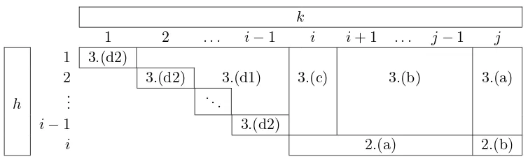
Figure 1. A sketch for the matrixΞi in equation (31).
For any 1 ≤ h ≤ n, such a matrix with the index h written below has α1(i) rows and α(1h)
columns. Let for any natural numbersaand b denote 0a×b thea×bzero matrix. According to equation (29), we have
[Ξi]h = (
−✶α(i) 1
, h=i,
0α(i) 1 ×α
(h) 1
, h6=i.
Using the matrices [Ξi]h and [Ξi]h as blocks, we now build the matrix
Ξi =
[Ξi]1 [Ξi]2· · · [Ξi]n [Ξi]1 [Ξi]2· · · [Ξi]n
.
Taking into account what we have noted on its entries, this means
Ξi =
[Ξi]1 · · · [Ξi]i−1 [Ξi]i 0· · ·0 0 · · · 0 −✶α(i)
1
0· · ·0 !
. (31)
A sketch of such a matrix Ξi where the entries which may be different from zero are marked as shaded areas and −✶α(i)
1
as a diagonal line is given in Fig. 1.
For allh where 1≤h≤n, we call the block [Ξi]h inΞi stacked upon the block [Ξi]h inΞi the hth block of columns in Ξi. For those h with β1(h) =m thehth block of columns is empty.
Now the symbol fields ¯Yhβ, or equivalently the pairs (β, h)6∈ B, are used to order the dimN1=r
columns of Ξi, according to increasing h into n blocks (empty for those h with α(1h) = 0) and within each block according to increasingβ (with β1(j)+ 1≤β ≤m).
Remark 4. This means, the columns in Ξi are ordered increasingly with respect to the term-over-position lift of the degree reverse lexicographic ranking. Therefore, the entry−Ch
β(h)1 +γ(φ α i) stands in the matrix Ξi in line α, in the hth block of columns of which it is the γth one from the left. Entries different from zero and from −1 may appear in Ξi only in a [Ξi]h for h ≤i. To be exact, for any classi, the matrixΞi hasα(1i) rows where all entries are zero with only one exception: for each 1≤ℓi < α(1i) we have
Ξβ
(i) 1 +ℓi
where ℓ := Pih−=11 α(1h)+ℓi. The entries in the remaining upper β(1i) rows are −Cβh(φαi). The potentially non-trivial ones of them are marked as shaded areas in Fig. 1.
Note that for a differential equation with constant coefficients all vectorsΘij vanish and for a maximally over-determined equation there are no matrices Ξi.
The unit block ofα(1i) rows, ✶α(i) 1
, leads immediately to the estimate
α(1i)≤rankΞi≤min (
m,
i X
h=1
α(1h)
)
.
Example 5. For Example 1, we have n = 2 and therefore two matrices Ξ1 and Ξ2. Their
entries follow immediately from our results in Example 4. Fori= 1, we have
Ξ1 =
0 0
−1 0 0 −1
.
The first line is [Ξ1]1= (0,0). The unit block below it is [Ξ1]1. (We haveβ1(1) = 1 and therefore
α(1)1 = 2. There is only h = 1 to consider, as both parametric derivatives vx and wx are with respect toxonly.) Because of the very simple nature of our system, we find here by accident that
Ξ1 =Ξ2. However, [Ξ2]1=Ξ2 is the whole matrix while there is no [Ξ2]1 becauseβ(2)1 =m= 3
and therefore α(2)1 = 0. Finally, we obtain Θ12 = (vx−wt,0,0)t. (The t top right marks the transpose.) Note that its first entry is in fact the integrability condition.
6
Flat Vessiot connections
In this section, we develop an approach for constructing flat Vessiot connections which improves recent approaches [5, 24, 27]: we exploit the splitting of V[Rq] suggested by (23) to introduce convenient bases for integral distributions which yield structure equations that are particularly simple. Finally, we give necessary and sufficient conditions for Vessiot’s approach to succeed.
Let Rq locally be represented by the system Φτ(x,u(q)) = 0 where 1 ≤ τ ≤ t. Our goal is the construction of all n-dimensional transversal involutive subdistributions U within the Vessiot distribution V[Rq]. Taking for the Vessiot distribution the basis (Xi, Yk) where the vector fieldsYkare the above mentioned basis of the symbolT ι(Nq) with vanishing Lie brackets and the vector fields Xi are given in (25), we make for the basis (Ui: 1 ≤ i ≤ n) of such a subdistributionU the ansatz
Ui =Xi+ζikYk
with yet undetermined coefficient functions ζk
i ∈ F(Rq). This ansatz follows naturally from our considerations so far, as the fields Xi are transversal to the fibration over X and span a reference complement to the symbol and inNq all fields Yk are vertical.
Since the fieldsUi are in triangular form, the distributionU is involutive if, and only if, their Lie brackets vanish, and using the structure equations (26) this means:
[Ui, Uj] = [Xi, Xj] +ζik[Yk, Xj] +ζjk[Xi, Yk] + Ui(ζjk)−Uj(ζik)
Yk = Θijc −Ξjkc ζik+Ξikc ζjk
Zc+ Ui(ζjk)−Uj(ζik)
Yk= 0. (32)
of conditions for the coefficient functions ζk
i: a system of algebraic equations
Gcij :=Θcij−Ξjkc ζik+Ξikc ζjk= 0,
1≤c≤C,
1≤i < j ≤n, (33)
and a system of differential equations
Hijp :=Ui(ζjp)−Uj(ζip) = 0,
1≤p≤r,
1≤i < j ≤n. (34)
In the algebraic system (33) the true structure coefficientsΘc
ij,Ξjkc appear. For our subsequent analysis we follow Remark2and replace them by the extended set of coefficientsΘα
ij,Ξjkα. This corresponds to replacing (33) by an equivalent but larger linear system of equations which is, however, simpler to analyse.
Obviously, (33) is an inhomogeneouslinear system to which any solution method for linear systems can be applied. We shall see in the next section that its structure (induced by the structure equations of the Vessiot distribution) allows us to decompose it into simpler subsystems which are considered step by step. Many papers on the Vessiot theory (see for example [5,24]) study at this stage a quadratic system which only by such a step-by-step approach can be reduced to a series of linear problems. The linearity of (33) is a simple consequence of our choice of a basis for V[Rq] which in turn exploits the natural splittingV[Rq] =Nq⊕ H.
Remark 5. The vector fields Yk lie in the Vessiot distribution V[R1]. Thus, according to
Proposition5, the subdistributionU is an integral distribution if, and only if, the coefficientsζi k satisfy the algebraic conditions (33). This observation permits us immediately to reduce the number of unknowns in our ansatz. Assume that we have values 1 ≤i, j ≤ nand 1 ≤α ≤m
such that both (α, i) and (α, j) are not contained in B, that is, uα
i and uαj are both parametric derivatives (and thus obviously the second-order derivative uα
ij, too). Then there exist two symbol fields Yk = ι∗(∂uα
i) and Yl = ι∗(∂uαj). Now it follows from the coordinate form (3) of the contact map that the subdistribution U, spanned by the vector fields Uh =Xh+ζhkYk for 1≤h≤n, can be an integral distribution if, and only if,
ζjk=ζil or, equivalently, ζ
(α,i)
j =ζ
(α,j)
i . (35)
for all 1≤i < j ≤nand 1≤k, l≤r. As the unknowns ζk
j may be understood as labels for the columns of the matrices Ξh, this identification leads to a contraction of these matrices. The contracted matrices, denoted by
ˆ
Ξh, arise as follows: whenever ζjk =ζil then the corresponding columns of Ξh are added; their sum replaces the first of these columns, while the second column is dropped. Similarly, we introduce reduced vectors ˆζh where the redundant components are left out. From now on, we always understand that in the equations above this reduction has been performed. Otherwise some results would not be correct (see Example 10 below).
For a more thorough outline of these technical details, see [6, Lemma 3.3.5 and Remark 3.3.6].
Example 6. We consider a first-order equation in one dependent variable
R1:
un=φn(x, u, u1, . . . , un−r−1),
· · · ·
un−r=φn−r(x, u, u1, . . . , un−r−1).
the indices: 1 ≤ k, ℓ < n−r and n−r ≤ a, b ≤ n. Thus we may express our system in the concise formua=φa(x, u, uk) and local coordinates on the submanifoldR1 are (x, u, uk).
The pull-back of the contact formω=du−uidxi generating the contact codistributionC10 is
ι∗ω=du−ukdxk−φadxa and V[R1] =hX¯1, . . . ,X¯n,Y¯1, . . . ,Y¯n−r−1i where
¯
Xk=∂xk+uk∂u, X¯a=∂xa+φa∂u, Y¯k =∂u k.
The fields ¯Yk span the symbol N1 and the fields ¯Xi our choice of a reference complement H0.
Setting ¯Z =∂u, the structure equations ofV[R1] are
[ ¯Xk,X¯ℓ] = 0, [ ¯Yk,Y¯ℓ] = 0,
[ ¯Xk,X¯a] = ¯Xk(φa) ¯Z, [ ¯Xa,X¯b] = X¯a(φb)−X¯b(φa) ¯
Z,
[ ¯Xk,Y¯ℓ] =−δkℓZ,¯ [ ¯Xa,Y¯k] =−Y¯k(φa) ¯Z.
Now we make the above discussed ansatzUi=Xi+ζikYk for the generators of a transversal complement H. Modulo the Vessiot distributionV[R1] we obtain for their Lie brackets
[Uk, Uℓ]≡(ζkℓ−ζℓk)Z modV[R1], (36a)
[Ua, Uk]≡ ζak−ζkℓYℓ(φa)−Xk(φa)
Z mod V[R1], (36b)
[Ua, Ub]≡ ζakYk(φb)−ζbℓYℓ(φa) +Xa(φb)−Xb(φa)
Z mod V[R1]. (36c)
The algebraic system (33) is now obtained by requiring that all the expressions in parentheses on the right hand sides vanish. Its solution is straightforward. The first subsystem (36a) implies the equalities ζℓ
k=ζℓk. This result was to be expected by the discussion in Remark 5: both uk anduℓ are parametric derivatives forR1and thus we could have made this identification already
in our ansatz for the complement. The second subsystem (36b) yields that ζk
a = ζkℓYℓ(φa) +
Xk(φa). If we enter these results into the third subsystem (36c), then all unknowns ζ drop out and the solvability condition
Xa(φb)−Xb(φa) +Xk(φa)Yk(φb)−Xk(φb)Yk(φa) = 0
arises. Thus in this example the algebraic system (33) has a solution if, and only if, this condition is satisfied.
Comparing with the classical theory of such systems, one easily verifies that this solvability condition is equivalent to the vanishing of the Mayer or Jacobi bracket [ua−φa, ub−φb] on the submanifoldR1, which in turn is a necessary and sufficient condition for the formal integrability
of the differential equationR1. Thus we may conclude thatR1 possessesn-dimensional integral
distributions if, and only if, it is formally integrable (which in our case is also equivalent to R1
being involutive).
Thus here involution can be decided solely on the basis of the algebraic system (33). We will show in the next section that this observation does not represent a special property of a very particular class of differential equations but a general feature of the Vessiot theory.
7
The existence theorem for integral distributions
Now the question arises, when the combined system (33), (34) has solutions? We begin by analysing the algebraic part (33). We use for this analysis a step-by-step approach originally proposed by Vessiot [28]. Our analysis will automatically reveal necessary and sufficient assump-tions for it to succeed. As outlined in Remark 5, we replace ζ2 by ˆζ2 since for the entriesζ2(β,1)
the construction of the integral distributionU by first choosing an arbitrary vector fieldU1 and
then aiming for another vector fieldU2 such that [U1, U2]∈T ι(V[Rq]). During the construction of the field U2 we regard the components of the vector ζ1 = ˆζ1 as given parameters and the
components of ˆζ2 as the only unknowns of the system
ˆ
Ξ1ζˆ2= ˆΞ2ζˆ1−Θ12. (37)
Since the components of ˆζ1 are not considered unknowns, the system (37) must not lead to any
restrictions for the coefficients ˆζ1k. Obviously, this is the case if, and only if,
rank ˆΞ1 = rank ( ˆΞ1 Ξˆ2). (38)
Assuming that (38) holds, the system (37) is solvable if, and only if, it satisfies the augmented rank condition
rank ˆΞ1 = rank ( ˆΞ1 Ξˆ2 −Θ12). (39)
When we have succeeded in constructing U2, the next step is to seek a further vector fieldU3
such that [U1, U3]∈ T ι(V[Rq]) and [U2, U3]∈T ι(V[Rq]). Now the components of both vectors
Now this system is not to restrict the components of both ˆζ1 and ˆζ2 any further. The
interrela-tions between the ˆζi following from the condition (35) for the existence of integral distributions, given in Remark5, are taken care of by contractingΞ3 into ˆΞ3. This implies that now the rank
condition
is solvable if, and only if, the augmented rank condition
rank
form spanning an involutive subdistribution ofT ι(V[R1]), we construct the next vector fieldUj by solving the system
Assuming that it holds, the equations (40) are solvable and yield solutions for the components of ˆζj if, and only if, the system satisfies the augmented rank condition
rank
Remark 6. We can simplify our calculations for a differential equation Rq, represented by
uα
µ=φαµ(x,u,uˆ(q)) where each equation is solved for a principal derivative (all pairwise different)
uα
µ with |µ|=q, and where ˆu(q) denotes the set of the remaining, thus parametric, derivatives of order q and less. (Example 1 discusses a system of that kind.) Now we can use the local coordinates onRq. For the generators of the symbolNqwe may choose for (α, µ)6∈ B the vector
which satisfy equation (27). For the vector fields Wa which appear in equation (25) we may choose the contact vector fields Cαµ where (α, µ)∈ B. The further procedure, solving first the structure equations, which now take the simple form (26), to find the generators ofV′(R
q) and then solving equation (33) for the coefficient functions ζj, is the same as in the case where the representation is not in the above solved form.
Example 7. Before we proceed with our theoretical analysis, let us demonstrate with a concrete differential equation that in general we cannot expect that the above outlined step-by-step construction of integral distributions works. In order to keep the size of the example reasonably small, we use the second-order equation1 R
2 defined by the system uxx = αu and uyy = βu with two real constants α, β. Its symbolN2 is not involutive. However, one easily proves that
R2 is formally integrable for arbitrary choices of the constantsα,β. One readily computes that
the Vessiot distributionV[R2] is generated by the following three vector fields on R2:
X1=∂x+ux∂u+αu∂ux +uxy∂uy, X2 =∂y+uy∂u+uxy∂ux+βu∂uy, Y1 =∂uxy.
They yield as structure equations for V[R2]:
[X1, X2] =βux∂uy−αuy∂ux, [X1, Y1] =−∂uy, [X2, Y1] =−∂ux.
For the construction of a two-dimensional integral distributionU ⊂ V[R2] we make as above
the ansatz Ui = Xi+ζi1Y1 with two coefficients ζi1. As we want to perform a step-by-step construction, we assume that we have chosen some fixed value forζ1
1 and try now to determineζ21
such that [U1, U2]≡0 modV[R2]. Evaluation of the Lie bracket yields the equation
[U1, U2]≡(βux−ζ21)∂uy−(αuy−ζ
1
1)∂ux mod V[R2]. (43)
A necessary condition for the vanishing of the right side is that ζ1
1 = αuy. Hence one cannot choose this coefficient arbitrarily, as we assumed, but (43) determinesbothfunctionsζi1uniquely. Note that the conditions on the coefficientsζi1 imposed by (43) are trivially solvable and thusR2
possesses an integral distribution (which is even involutive). The problem is that it could not be constructed systematically with the above outlined step-by-step process.
1It could always be rewritten as a first-order one satisfying the assumptions made above, and the phenomenon
The following theorem links the satisfaction of the rank conditions (41) and (42), and thus the solvability of the algebraic system (33) by the above described step-by-step process, with intrinsic properties of the differential equationRq and its symbolNq. It represents an existence theorem for integral distributions.
Theorem 2. Assume that δ-regular coordinates have been chosen for the local representation of the differential equation Rq. Then the rank condition (41) is satisfied for all 1≤j ≤nif, and only if, the symbol Nq is involutive. The augmented rank condition (42) holds for all 1≤j≤n if, and only if, the differential equation Rq is involutive.
The proof of Theorem2 is given in AppendixA, as parts of it are rather technical. First, we transform the differential equation into an equivalent first-order system with a representation in the reduced Cartan normal form (10) and the same Cartan characters. This is always possible; see, for example, [23, Proposition A.3.1]. The basic idea of the proof is then that the rank condition (41) is equivalent to the vanishing of the obstructions to involution of the symbol in Lemma2, and the augmented rank condition (42) is equivalent to the vanishing of the remaining integrability conditions (recall that Lemma2gives all obstructions to involution only if the used coordinates are δ-regular so that this assumption is necessary in Theorem 2). The concrete implementation of this idea requires some technical considerations concerning the transformation of the matrices (41) and (42) into row echelon form, working out their contractions and analysing the interrelation between these operations.
Example 8. We demonstrate the role ofδ-regularity of the coordinates with the wave equation
uxy = 0 in characteristic coordinates which are not δ-regular. A straightforward computation yields as generators for the Vessiot distribution the fields X1 = C1(2), X2 = C2(2), Y1 = ∂uxx and Y2 = ∂uyy. Following our approach, we make the ansatz U1 = X1 +ζ11Y1 +ζ12Y2 and
U2 =X2+ζ21Y1+ζ22Y2. Evaluation of the Lie bracket [U1, U2] yields now the algebraic equations
ζ12= 0 andζ21 = 0 and the differential equationsU1(ζ21)−U2(ζ11) = 0 andU1(ζ22)−U2(ζ12) = 0.
As in Example 7, we see that the step-by-step process is broken, since we obtain a condition on the coefficientζ2
1 = 0 which we should be able to consider a parameter here.
At this point, we have proven that integral distributions within the Vessiot distribution exist if, and only if, the algebraic conditions (33) are solvable, and that this is equivalent to the augmented rank condition (41) being satisfied. This in turn is the case precisely if the differential equation is involutive. Thus we have characterised the existence of Vessiot connections for Vessiot’s [28] step-by-step approach.
8
The existence theorem for f lat Vessiot connections
There remains to analyse the solvability, if we add the differential system (34). Its solvability is equivalent to the existence of flat Vessiot connections in that each flat Vessiot connection ofR1 corresponds to a solution of the combined system (33), (34). We first note that the set of
differential conditions (34) alone is again an involutive system.
Proposition 7. The differential conditions (34) alone represent an involutive differential equa-tion of first order.
The proof, which is somewhat technical, is given in AppendixB. It is based on an evaluation of the Jacobi identity for the Lie brackets of the fields Ui.
If the original equationR1is analytic, then the quasi-linear system (34) is analytic, too. Thus