PRACTICAL
GRAPH MINING
WITH R
Chapman & Hall/CRC
Data Mining and Knowledge Discovery Series
PUBLISHED TITLES
SERIES EDITOR
Vipin Kumar
University of MinnesotaDepartment of Computer Science and Engineering Minneapolis, Minnesota, U.S.A.
AIMS AND SCOPE
This series aims to capture new developments and applications in data mining and knowledge discovery, while summarizing the computational tools and techniques useful in data analysis. This series encourages the integration of mathematical, statistical, and computational methods and techniques through the publication of a broad range of textbooks, reference works, and hand-books. The inclusion of concrete examples and applications is highly encouraged. The scope of the series includes, but is not limited to, titles in the areas of data mining and knowledge discovery methods and applications, modeling, algorithms, theory and foundations, data and knowledge visualization, data mining systems and tools, and privacy and security issues.
ADVANCES IN MACHINE LEARNING AND DATA MINING FOR ASTRONOMY
Michael J. Way, Jeffrey D. Scargle, Kamal M. Ali, and Ashok N. Srivastava
BIOLOGICAL DATA MINING
Jake Y. Chen and Stefano Lonardi
COMPUTATIONAL INTELLIGENT DATA ANALYSIS FOR SUSTAINABLE DEVELOPMENT
Ting Yu, Nitesh V. Chawla, and Simeon Simoff
COMPUTATIONAL METHODS OF FEATURE SELECTION
Huan Liu and Hiroshi Motoda
CONSTRAINED CLUSTERING: ADVANCES IN ALGORITHMS, THEORY, AND APPLICATIONS
Sugato Basu, Ian Davidson, and Kiri L. Wagstaff
CONTRAST DATA MINING: CONCEPTS, ALGORITHMS, AND APPLICATIONS
Guozhu Dong and James Bailey
DATA CLUSTERING: ALGORITHMS AND APPLICATIONS
Charu C. Aggarawal and Chandan K. Reddy
DATA CLUSTERING IN C++: AN OBJECT-ORIENTED APPROACH
Guojun Gan
DATA MINING FOR DESIGN AND MARKETING
Yukio Ohsawa and Katsutoshi Yada
DATA MINING WITH R: LEARNING WITH CASE STUDIES
Luís Torgo
FOUNDATIONS OF PREDICTIVE ANALYTICS
James Wu and Stephen Coggeshall
GEOGRAPHIC DATA MINING AND KNOWLEDGE DISCOVERY, SECOND EDITION
Harvey J. Miller and Jiawei Han
HANDBOOK OF EDUCATIONAL DATA MINING
Cristóbal Romero, Sebastian Ventura, Mykola Pechenizkiy, and Ryan S.J.d. Baker
INTELLIGENT TECHNOLOGIES FOR WEB APPLICATIONS
Priti Srinivas Sajja and Rajendra Akerkar
INTRODUCTION TO PRIVACY-PRESERVING DATA PUBLISHING: CONCEPTS AND TECHNIQUES
Benjamin C. M. Fung, Ke Wang, Ada Wai-Chee Fu, and Philip S. Yu
KNOWLEDGE DISCOVERY FOR COUNTERTERRORISM AND LAW ENFORCEMENT
David Skillicorn
KNOWLEDGE DISCOVERY FROM DATA STREAMS
João Gama
MACHINE LEARNING AND KNOWLEDGE DISCOVERY FOR ENGINEERING SYSTEMS HEALTH MANAGEMENT
Ashok N. Srivastava and Jiawei Han
MINING SOFTWARE SPECIFICATIONS: METHODOLOGIES AND APPLICATIONS
David Lo, Siau-Cheng Khoo, Jiawei Han, and Chao Liu
MULTIMEDIA DATA MINING: A SYSTEMATIC INTRODUCTION TO CONCEPTS AND THEORY
Zhongfei Zhang and Ruofei Zhang
MUSIC DATA MINING
Tao Li, Mitsunori Ogihara, and George Tzanetakis
NEXT GENERATION OF DATA MINING
Hillol Kargupta, Jiawei Han, Philip S. Yu, Rajeev Motwani, and Vipin Kumar
PRACTICAL GRAPH MINING WITH R
Nagiza F. Samatova, William Hendrix, John Jenkins, Kanchana Padmanabhan, and Arpan Chakraborty
RELATIONAL DATA CLUSTERING: MODELS, ALGORITHMS, AND APPLICATIONS
Bo Long, Zhongfei Zhang, and Philip S. Yu
SERVICE-ORIENTED DISTRIBUTED KNOWLEDGE DISCOVERY
Domenico Talia and Paolo Trunfio
SPECTRAL FEATURE SELECTION FOR DATA MINING
Zheng Alan Zhao and Huan Liu
STATISTICAL DATA MINING USING SAS APPLICATIONS, SECOND EDITION
George Fernandez
SUPPORT VECTOR MACHINES: OPTIMIZATION BASED THEORY, ALGORITHMS, AND EXTENSIONS
Naiyang Deng, Yingjie Tian, and Chunhua Zhang
TEMPORAL DATA MINING
Theophano Mitsa
TEXT MINING: CLASSIFICATION, CLUSTERING, AND APPLICATIONS
Ashok N. Srivastava and Mehran Sahami
THE TOP TEN ALGORITHMS IN DATA MINING
Xindong Wu and Vipin Kumar
UNDERSTANDING COMPLEX DATASETS: DATA MINING WITH MATRIX DECOMPOSITIONS
David Skillicorn
This page intentionally left blank
This page intentionally left blank
PRACTICAL
GRAPH MINING
WITH R
Edited by
Nagiza F. Samatova
William Hendrix
John Jenkins
Kanchana Padmanabhan
Arpan Chakraborty
Taylor & Francis Group
6000 Broken Sound Parkway NW, Suite 300 Boca Raton, FL 33487-2742
© 2014 by Taylor & Francis Group, LLC
CRC Press is an imprint of Taylor & Francis Group, an Informa business
No claim to original U.S. Government works Version Date: 20130722
International Standard Book Number-13: 978-1-4398-6085-4 (eBook - PDF)
This book contains information obtained from authentic and highly regarded sources. Reasonable efforts have been made to publish reliable data and information, but the author and publisher cannot assume responsibility for the validity of all materials or the consequences of their use. The authors and publishers have attempted to trace the copyright holders of all material reproduced in this publication and apologize to copyright holders if permission to publish in this form has not been obtained. If any copyright material has not been acknowledged please write and let us know so we may rectify in any future reprint.
Except as permitted under U.S. Copyright Law, no part of this book may be reprinted, reproduced, transmit-ted, or utilized in any form by any electronic, mechanical, or other means, now known or hereafter inventransmit-ted, including photocopying, microfilming, and recording, or in any information storage or retrieval system, without written permission from the publishers.
For permission to photocopy or use material electronically from this work, please access www.copyright. com (http://www.copyright.com/) or contact the Copyright Clearance Center, Inc. (CCC), 222 Rosewood Drive, Danvers, MA 01923, 978-750-8400. CCC is a not-for-profit organization that provides licenses and registration for a variety of users. For organizations that have been granted a photocopy license by the CCC, a separate system of payment has been arranged.
Trademark Notice: Product or corporate names may be trademarks or registered trademarks, and are used only for identification and explanation without intent to infringe.
Visit the Taylor & Francis Web site at http://www.taylorandfrancis.com
and the CRC Press Web site at http://www.crcpress.com
List of Figures ix
List of Tables xvii
Preface xix
1 Introduction 1
Kanchana Padmanabhan, William Hendrix, and Nagiza F. Samatova
2 An Introduction to Graph Theory 9
Stephen Ware
3 An Introduction to R 27
Neil Shah
4 An Introduction to Kernel Functions 53
John Jenkins
5 Link Analysis 75
Arpan Chakraborty, Kevin Wilson, Nathan Green, Shravan Kumar Alur, Fatih Ergin, Karthik Gurumurthy, Romulo Manzano, and Deepti Chinta
6 Graph-based Proximity Measures 135
Kevin A. Wilson, Nathan D. Green, Laxmikant Agrawal, Xibin Gao, Dinesh Madhusoodanan, Brian Riley, and James P. Sigmon
7 Frequent Subgraph Mining 167
Brent E. Harrison, Jason C. Smith, Stephen G. Ware, Hsiao-Wei Chen, Wenbin Chen, and Anjali Khatri
8 Cluster Analysis 205
Kanchana Padmanabhan, Brent Harrison, Kevin Wilson, Michael L. Warren, Katie Bright, Justin Mosiman, Jayaram Kancherla, Hieu Phung, Benjamin Miller, and Sam Shamseldin
vii
9 Classification 239 Srinath Ravindran, John Jenkins, Huseyin Sencan, Jay Prakash Goel, Saee Nirgude, Kalindi K Raichura, Suchetha M Reddy, and Jonathan S. Tatagiri
10 Dimensionality Reduction 263
Madhuri R. Marri, Lakshmi Ramachandran, Pradeep Murukannaiah, Padmashree Ravindra, Amrita Paul, Da Young Lee, David Funk, Shanmugapriya Murugappan, and William Hendrix
11 Graph-based Anomaly Detection 311
Kanchana Padmanabhan, Zhengzhang Chen, Sriram
Lakshminarasimhan, Siddarth Shankar Ramaswamy, and Bryan Thomas Richardson
12 Performance Metrics for Graph Mining Tasks 373
Kanchana Padmanabhan and John Jenkins
13 Introduction to Parallel Graph Mining 419
William Hendrix, Mekha Susan Varghese, Nithya Natesan, Kaushik Tirukarugavur Srinivasan, Vinu Balajee, and Yu Ren
Index 465
2.1 An example graph. . . 10
2.2 An induced subgraph. . . 13
2.3 An example isomorphism and automorphism. . . 14
2.4 An example directed graph. . . 16
2.5 An example directed graph. . . 17
2.6 An example tree. . . 19
2.7 A directed, weighted graph. . . 20
2.8 Two example graphs, an undirected version (A) and a directed version (B), each with its vertices and edges numbered. . . . 21
2.9 Problems 1 and 2 refer to this graph. . . 24
2.10 Problem 3 refers to these graphs. . . 24
4.1 An example dataset. On the left, a class assignment where the data can be separated by a line. On the right, a class assignment where the data can be separated by an ellipse. . 54
4.2 The example non-linear dataset from Figure 4.1, mapped into a three-dimensional space where it is separable by a two-dimensional plane. . . 55
4.3 A: Analysis on some unmodified vector data. B: Analysis on an explicit feature space, using the transformationφ. C: Analysis on an implicit feature space, using the kernel functionk, with the analysis modified to use only inner products. . . 57
4.4 Three undirected graphs of the same number of vertices and edges. How similar are they? . . . 60
4.5 Three graphs to be compared through walk-based measures. The boxed in regions represent vertices more likely to be vis-ited in random walks. . . 63
4.6 Two graphs and their direct product. . . 63
4.7 A graph and its 2-totter-free transformation. . . 67
4.8 Kernel matrices for problem 1. . . 71
4.9 Graph used in Problem 9 . . . 72
5.1 Link-based mining activities. . . 79
5.2 A randomly generated 10-node graph representing a synthetic social network. . . 84
5.3 The egocentric networks for nodes 9 and 7. . . 88
ix
5.4 The egocentric network of node 1. . . 89
5.5 The egocentric network of node 6. . . 89
5.6 A five web page network. . . 91
5.7 A randomly generated 20-node directed graph. . . 98
5.8 Depiction of nodes with their PageRank in the star graphg2. 99 5.9 HITS algorithm flow: web pages are preprocessed before hub and authority vectors are iteratively updated and normalized. 100 5.10 (a) A web page that points to many other web pages is known as a hub. (b) A web page that is pointed to by many other web pages is an authority. . . 101
5.11 A bipartite graph represents the most strongly connected group of vertices in a graph. Hubs and Authorities exhibit a mutually reinforcing relationship. . . 102
5.12 HITS preprocessing: an initial selection of web pages is grown to include additional related pages, encoded as a graph, and an adjacency matrix is generated. . . 102
5.13 Graph for the query “search engine,” run on the web. For illus-trative purposes, we consider six web pages, namely Bing.com, Google.com, Wikipedia.org, Yahoo.com, Altavista.com, and Rediffmail.com. . . 103
5.14 A graph with the core vertices in bold. . . 112
5.15 Diagram depicting the test set and the newly predicted edges among the verticesA, B, C, andF (core vertices). . . 113
5.16 High-level abstraction of the link prediction process. . . 118
5.17 Pruned co-authorship network. . . 123
5.18 A simple graph for Question 10. . . 129
5.19 A simple graph for Question 11. . . 129
5.20 A graph for Question 12. . . 130
5.21 A graph for Question 13. . . 131
6.1 A high-level overview of the SNN algorithm described in detail in Algorithm 6. . . 139
6.2 Example proximity graph in which vertices are similar only if they are connected by an edge. . . 140
6.3 Proximity graph to show proximity based on vertices sharing neighbors. . . 140
6.4 The KNN graph obtained from the proximity matrix in Table 6.3 andk= 2. . . 141
6.5 Undirected graph of web page links for SNN proximity mea-sure. . . 142
6.6 Graph illustrating the results of the SNN Algorithm applied to the graph shown in Figure 6.5, withk= 2. . . 144
6.7 A KNN graph. . . 144
6.9 Figure indicating the ability of shared nearest neighbor to
form links between nodes in different clusters. . . 146
6.10 Directed graph to model journal article citations, where each edge indicates citations of one article by another. For example, articlen5 cites both articlesn1 andn2. . . 147
6.11 Bibliographic coupling graph (A) and co-citation graph (B) for the citation graph in Figure 6.10. . . 149
6.12 A high-level overview of the Neumann Kernel algorithm de-scribed in detail in Algorithm 7. . . 156
6.13 Example graph for Exercise 2. . . 163
6.14 Example graph for Exercise 3. . . 163
6.15 Example graph for Exercise 6. . . 165
7.1 This database consists of four chemicals represented as graphs based on their molecular structure. The hydroxide ion is fre-quent because it appears in three of the four graphs. Depend-ing on howsupport is defined, the support of hydroxide may be considered to be 0.75 or 3. . . 168
7.2 Possible gSpan Encodings of a sample graph (at left). The vertices are numbered according to their depth-first traversal ordering. Copyright ©IEEE. All rights reserved. Reprinted with permission, from [13] . . . 174
7.3 Graph growth: Rightmost extension to subgraphs. . . 175
7.4 gSpan can avoid checking candidates that are isomorphic to ones it has already or will eventually consider. . . 176
7.5 Example graphs on which gSpan will operate. . . 177
7.6 Example: the procedure of discovering subgraphs. . . 178
7.7 GraphBis a compression of graphA. GraphAhas 9 vertices and 11 edges. Notice that there are three triangles in graph A. If the triangle is encoded just once, each of the three tri-angles can be replaced with a pointer to that single triangle, reducing the number of vertices in graphBto 3 and the num-ber of edges to 2. Some extra space will be needed to store the representation of one triangle, but overall, graphB has a more compact representation. . . 181
7.8 The example graph for SUBDUE. . . 184
7.9 The frequent subgraphs discovered by SUBDUE. . . 185
7.11 Label-preserving automorphisms of the same unordered tree.
The integers shown represent preorder traversal positions. . 189
7.12 Child and cousin extension formed by adding a vertex with labelB as a child or cousin of vertex 4, denotedP4 B. . . 190
7.13 A match label identifies corresponding vertex positions for a subtree in its containing tree. . . 191
7.14 Example: a small collection of html documents. . . 192
7.15 The pinwheel graph. . . 200
7.16 Frequent subgraphs discovered by SUBDUE from Figure 7.15. 200 7.17 gSpan encodings graph. . . 201
7.18 A match label identifies corresponding vertex positions for a subtree in its containing tree. . . 202
8.1 An example of Prim’s algorithm for finding a minimum span-ning tree in the graph. . . 209
8.2 Clustering the minimum spanning tree in Figure 8.1. . . 210
8.3 Jarvis-Patrick clustering on unweighted graphs. . . 213
8.4 Examples for vertex and edge betweenness. . . 214
8.5 Example normalized centrality calculations. . . 218
8.6 Unweighted graph (G) used in the HCS clustering example. 220 8.7 The BK algorithm applied on an example graph. . . 223
8.8 GraphGused in the maximal clique enumeration R example. 224 8.9 GraphGused in the graph-basedk-means R example. . . . 228
8.10 GraphGfor Exercise 1. . . 233
8.11 GraphGfor Question 8. . . 235
9.1 A binary data set which is linearly separable. . . 242
9.2 Two separating hyperplanes. Which one better encodes the trend of the data? . . . 242
9.3 A example hypergraph (G). . . 249
9.4 Two basic chemical structures. . . 253
9.5 Two basic chemical structures, as adjacency matrices. . . 253
9.6 Sample instances of molecule structures of different classes. 254 9.7 GraphsG1 andG2 in Problem 6 . . . 259
9.8 HypergraphH in Problem 9. . . 260
10.1 Graph representation of airport network with only five air-ports. . . 267
10.2 Graph representation of airport network with twenty different airports from the US and Canada. . . 267
10.3 A visual representation of the shortest paths in the airport example graph. . . 269
10.6 Thek-means clustering algorithm fails to identify the actual clusters in the circles dataset. . . 276 10.7 The data after kernel PCA has the desired characteristic of
linear separability. . . 277 10.8 A comparison between linear (MDS) and nonlinear (kernel
PCA) techniques for distinguishing between promising and not promising (underlined) customers for a telephone com-pany. . . 279 10.9 The figure on top depicts the principal components when
lin-ear PCA is carried out on the data. The principal component is represented by an arrow. The figure on the bottom shows the transformation of the data into a high-dimensional fea-ture space via a transformation Φ. The “kernel trick” helps us carry out this mapping of data with the help of kernel functions. Copyright @1998 Massachusetts Institute of Tech-nology. Reprinted with permission. All rights reserved. . . . 280 10.10 Thedirect product graph G=G1×G2, created fromG1 and
G2. . . 281
10.11 A high-level view of the steps involved in carrying out kernel PCA. . . 282 10.12 Experimental results for classifying diabetesdata using the
ldafunction in R. Large symbols represent the predicted class, whereas small symbols represent the actual class. The symbols are as follows: circles represent ‘chemical,’ triangles represent ‘normal,’ and pluses represent ‘overt.’ . . . 286 10.13 Overview of LDA presenting the flow of tasks in LDA. . . . 286 10.14 Within-class scatter and between-class scatter. . . 290 10.15 Graph representation of numerical example with two classes. 292 10.16 Plot of two clusters for clear cell patients (C) and non-clear
cell patients (N). The plots are generated using R. . . 299 10.17 Sample images used to demonstrate the application of LDA
for face recognition. . . 300
11.1 “White crow” and “in-disguise” anomalies. . . 313 11.2 Example of a pointwise anomaly. . . 313 11.3 Directed graph (a) and Markov transition matrix (b) for a
11.12 Probabilistic algorithm (GBAD-P) example. . . 336
11.13 Graph for maximum partial structure (GBAD-MPS) example. 338 11.14 A simple example of DBLP data. . . 340
11.15 A third-order tensor of network flow data. . . 341
11.16 The slices of a third-order tensor. . . 342
11.17 A third-order tensorχis matricized along mode-1 to a matrix X(1). . . 344
11.18 The third-order tensor χ[N1×N2×N3] ×1U results in a new tensor inRR×N2×N3. . . . 345
11.19 The Tucker decomposition. . . 347
11.20 Outline of the tensor-based anomaly detection algorithm. . . 349
11.21 A summary of the various research directions in graph-based anomaly detection. . . 361
11.22 GraphG1 for Question 1. . . 363
11.23 GraphG2 for Question 2a. . . 364
11.24 GraphG3 for Question 7. . . 366
11.25 GraphG4 for Question 9. . . 367
12.1 2×2 confusion matrix template for model M. A number of terms are used for the entry values, which are shown in i, ii, and iii. In our text we refer to the representation in Figure i. 375 12.2 Example of a 2×2 confusion matrix. . . 376
12.3 Multi-level confusion matrix template. . . 382
12.4 Example of a 3×3 confusion matrix. . . 382
12.5 Multi-level matrix to a 2×2 conversion. . . 383
12.6 Expected confusion matrix. . . 385
12.7 An example of expected and observed confusion matrices. . 385
12.8 ROC space and curve. . . 391
12.9 Plotting the performance of three models, M1, M2, and M3 on the ROC space. . . 392
12.10 Contingency table template forprior knowledge based evalu-ation. . . 395
12.11 Contingency table example forprior knowledge based evalu-ation. . . 395
12.12 Matching matrix template for prior knowledge based evalua-tion. . . 397
12.13 Matching matrix example. . . 397
12.14 Example of a pair of ideal and observed matrices. . . 400
12.15 Cost matrix template for model comparison. . . 406
13.1 Some of the major sources of overhead: (a) Initialization of the parallel environment, (b) Initial data distribution, (c) Com-munication costs, (d) Dependencies between processes, (e) Synchronization points, (f) Workload imbalances, (g) Work duplication, (h) Final results collection, (i) Termination of the parallel environment. . . 422 13.2 The diagram above explains the fundamental working
prin-ciple behind the embarrassingly parallel computation. The figure illustrates a simple addition of array elements using embarrassingly parallel computing. . . 423 13.3 Division of work required to build a house. . . 424 13.4 Basic illustration of embarrassingly parallel computation. . . 426 13.5 Some of the possible sources of overhead for the mclapply
function: (a) Setting up the parallel environment/distributing data (spawningthreads), (b) Duplicated work (if, say, dupli-cates exist in the list), (c) Unbalanced loads (from uneven distribution or unequal amounts of time required to evaluate the function on a list item), (d) Combining results/shutting down the parallel environment. . . 428 13.6 A simple strategy for parallel matrix multiplication. . . 429 13.7 Strategy for parallelizing the double centering operation. . . 431 13.8 Some of the different ways to call parallel codes from R. . . 432 13.9 Work division scheme for calculating matrix multiplication
in RScaLAPACK. The matrix is divided into NPROWS rows andNPCOLScolumns, and the resulting blocks are distributed among the processes. Each process calculates the product for its assigned block, and the results are collected at the end. . 434 13.10 Basic strategy for transformingcmdscaleto parallelcmdscale.
435
13.11 Overview of the three main parts of master-slave program-ming paradigm. . . 437 13.12 The figure above shows a process Pi communicating with a
single processPj. . . 440
13.13 A basic illustration ofmpi.bcastis shown in the above figure: processPi sends a copy of the data to all of the other processes. 445
13.14 The above figure shows how a vector is evenly divided among four processes. Each process will receive a part of the vector. 445 13.15 The above figure shows how mpi.gather gathers each piece
of a large vector from different processes to combine into a single vector. . . 446 13.16 The above figure shows how mpi.reduce collects the results
13.17 Results for running the parallel matrix multiplication code. Graph (a) shows the amount of time taken by the serial and parallel codes, and graph (b) shows the relative speedup for the different numbers of processes. The runs were performed on an 8-core machine, resulting in little or no speedup at the 16-process level. . . 454 13.18 Sample unbalanced (a) and balanced (b) workload
distribu-tions. In (a), the parallel algorithm would be limited by the time it takes process 3 to finish, whereas in (b), all of the pro-cesses would finish at the same time, resulting in faster overall computation. . . 455 13.19 Simulation results for solving a problem with an unbalanced
4.1 Some common kernel functions, for input vectorsxandy . 56
5.1 Top 10 social networking and blog sites: Total minutes spent by surfers in April 2008 and April 2009 (Source: Nielsen
NetView) . . . 82
5.2 PageRank Notation . . . 93
5.3 Parameters forpage.rank . . . 97
5.4 Adjacency matrix for web link data . . . 104
5.5 Convergence of authority scores,a, overkmaxiterations. Dec-imals have been rounded to three places. . . 108
5.6 Convergence of hub scores,h, over kmax iterations. Decimals have been rounded to three places. . . 108
5.7 Link prediction notation . . . 111
6.1 Glossary of terms used in this chapter . . . 137
6.2 Description of notation used in this chapter . . . 138
6.3 An example of a proximity matrix . . . 141
6.4 Adjacency matrix for the undirected proximity graph illus-trated in Figure 6.5 . . . 142
6.5 Term-document matrix for the sentences “I like this book” and “We wrote this book” . . . 151
6.6 Document correlation matrix for the sentences “I like this book” and “We wrote this book” . . . 152
6.7 Term correlation matrix for the sentences “I like this book” and “We wrote this book” . . . 152
6.8 Adjacency matrix for the directed graph in Figure 6.10 . . . 153
6.9 Authority and hub scores (from the HITS algorithm) for ci-tation data example in Figure 6.10 . . . 159
7.1 gSpan Encodings code for Fig. 7.2(a)-(c). . . 174
7.2 Textual representation of the input and output for the gSpan example . . . 177
7.3 Graph Compression . . . 181
7.4 SUBDUE Encoding Bit Sizes . . . 183
7.5 The number of potential labeled subtrees of a tree with up to five vertices and four labels is given by the formula in Equation 7.1. The configurations row indicates the number of possible node configurations for a tree of with k vertices, labellingsindicates the number of potential label assignments for a single configuration of a tree withkvertices, and candi-dates indicate the number of potential labeled subtrees for a
maximum tree size ofkvertices. . . 187
7.6 Example scope-list joins for treeT0 from Figure 7.10 . . . . 192
7.7 SLEUTH representation for the HTML documents in Fig-ure 7.14 . . . 193
7.8 Graph Compression . . . 201
10.1 Notations specific to this chapter . . . 265
10.2 Sample data from the diabetes dataset used in our example. The dataset contains 145 data points and 4 dimensions, in-cluding the class label. This dataset is distributed with the mclust package. . . 284
10.3 Confusion matrix for clustering using Euclidean distance that indicates 38 + 5 = 43 misclassified patients . . . 297
10.4 Confusion matrix for clustering using RF dissimilarity mea-sure that indicates 11 + 18 = 29 misclassified patients . . . . 298
11.1 Example dataset for cosine similarity . . . 316
11.2 Notations for random walk on a single graph . . . 317
11.3 Example 2: Vector representation of each node . . . 320
11.4 Notations for applying the random walk technique to multi-variate time series data (see Table 11.2 for notations on the single graph random walk technique) . . . 323
11.5 Notation for GBAD algorithms . . . 332
11.6 Table of notations for tensor-based anomaly detection . . . 343
11.7 Intrusion detection attributes . . . 352
11.8 Data for aDOS attack example . . . 353
11.9 Nokia stock market data attributes . . . 359
11.10 “Shared-Neighbor” matrix for Question 1 . . . 363
11.11 The predictor time seriesX for Question 6, with variables a andbmeasured at timest1,t2,t3, and t4 . . . 365
11.12 The target time seriesY for Question 6, with variablec mea-sured at timest1,t2,t3, and t4 . . . 366
12.1 Predictions by modelsM1andM2for Question 1 . . . 413
12.2 Cost matrix for Question 2 . . . 413
12.3 Data for Question 3 . . . 413
Graph mining is a growing area of study that aims to discover novel and insightful knowledge from data that is represented as a graph. Graph data is ubiquitous in real-world science, government, and industry domains. Examples include social network graphs, Web graphs, cybersecurity networks, power grid networks, and protein-protein interaction networks. Graphs can model the data that takes many forms ranging from traditional vector data through time-series data, spatial data, sequence data to data with uncertainty. While graphs can represent the broad spectrum of data, they are often used when links, relationships, or interconnections are critical to the domain. For example, in the social science domain, the nodes in a graph are people and the links between them are friendship or professional collaboration relationships, such as those captured by Facebook and LinkedIn, respectively. Extraction of useful knowledge from collaboration graphs could facilitate more effective means of job searches.
The book provides a practical, “do-it-yourself” approach to extracting in-teresting patterns from graph data. It covers many basic and advanced tech-niques for graph mining, including but not limited to identification of anoma-lous or frequently recurring patterns in a graph, discovery of groups or clusters of nodes that share common patterns of attributes and relationships, as well as extraction of patterns that distinguish one category of graphs from another and use of those patterns to predict the category for new graphs.
This book is designed as a primary textbook for advanced undergraduates, graduate students, and researchers focused on computer, information, and computational science. It also provides a handy resource for data analytics practitioners. The book is self-contained, requiring no prerequisite knowledge of data mining, and may serve as a standalone textbook for graph mining or as a supplement to a standard data mining textbook.
Each chapter of the book focuses on a particular graph mining task, such as link analysis, cluster analysis, or classification, presents three representa-tive computational techniques to guide and motivate the reader’s study of the topic, and culminates in demonstrating how such techniques could be utilized to solve a real-world application problem(s) using real data sets. Ap-plications include network intrusion detection, tumor cell diagnostics, face recognition, predictive toxicology, mining metabolic and protein-protein inter-action networks, community detection in social networks, and others. These representative techniques and applications were chosen based on availability of open-source software and real data, as the book provides several libraries
xix
for the R statistical computing environment to “walk-through” the real use cases. The presented techniques are covered in sufficient mathematical depth. At the same time, chapters include a lot of explanatory examples. This makes the abstract principles of graph mining accessible to people of varying lev-els of expertise, while still providing a rigorous theoretical foundation that is grounded in reality. Though not every available technique is covered in depth, each chapter includes a brief survey of bibliographic references for those inter-ested in further reading. By presenting a level of depth and breadth in each chapter with an ultimate focus on “hands-on” practical application, the book has something to offer to the student, the researcher, and the practitioner of graph data mining.
There are a number of excellent data mining textbooks available; however, there are a number of key features that set this book apart. First, the book focuses specifically on mining graph data. Mining graph data differs from traditional data mining in a number of critical ways. For example, the topic of classification in data mining is often introduced in relation to vector data; however, these techniques are often unsuitable when applied to graphs, which require an entirely different approach such as the use of graph kernels.
Second, the book grounds its study of graph mining in R, the open-source software environment for statistical computing and graphics (http://www.r-project.org/). R is an easy-to-learn open source software package for statistical data mining with capabilities for interactive, visual, and exploratory data analysis. By incorporating specifically designed R codes and examples directly into the book, we hope to encourage the intrepid reader to follow along and to see how the algorithmic techniques discussed in the book correspond to the process of graph data analysis. Each algorithm in the book is presented with its accompanying R code.
Third, the book is a self-contained, teach-yourself practical approach to graph mining. The book includes all source codes, many worked examples, exercises with solutions, and real-world applications. It develops intuition through the use of easy-to-follow examples, backed up with rigorous, yet ac-cessible, mathematical foundations. All examples can easily be run using the included R packages. The underlying mathematics presented in the book is self-contained. Each algorithmic technique is accompanied by a rigorous and formal explanation of the underlying mathematics, but all math preliminar-ies are presented in the text; no prior mathematical knowledge is assumed. The level of mathematical complexity ranges from basic to advanced topics. The book comes with several resources for instructors, including exercises and complete, step-by-step solutions.
1
Introduction
Kanchana Padmanabhan, William Hendrix North Carolina State University
Nagiza F. Samatova
North Carolina State University and Oak Ridge National Laboratory
CONTENTS
1.1 Graph Mining Applications . . . 2 1.2 Book Structure . . . 6
Recent years have been witnessing an explosion of graph data from a vari-ety of scientific, social, economic, and technological domains. In its simplest form, a graph is a collection of individual objects interconnected in some way. Examples include electric power grids connecting power grids across geograph-ically distributed locations, global financial systems connecting banks world-wide, and social networks linking individual users, businesses, or customers by friendship, collaboration, or transaction interactions.
Graph data analytics—extraction of insightful and actionable knowledge from graph data—shapes our daily life and the way we think and act. We often realize our dependence on graph data analytics only if failures occur in normal functioning of the systems that these graphs model and represent. A disruption in a local power grid can cause a cascade of failures in critical parts of the entire nation’s energy infrastructure. Likewise, a computer virus, in a blink of an eye, can spread over the Internet causing the shutdown of important businesses or leakage of sensitive national security information.
Intrinsic properties of these diverse graphs, such as particular patterns of interactions, can affect the underlying system’s behavior and function. Min-ing for such patterns can provide insights about the vulnerability of a nation’s energy infrastructure to disturbances, the spread of disease, or the influence of people’s opinions. Such insights can ultimately empower us with actionable knowledge on how to secure our nation, how to prevent epidemics, how to increase efficiency and robustness of information flow, how to prevent catas-trophic events, or how to influence the way people think, form opinions, and act.
Graphs are ubiquitous. Graph data is growing at an exponential rate.
Graph data analytics can unquestionably be very powerful. Yet, our ability to extract useful patterns, or knowledge, from graph data, to characterize intrinsic properties of these diverse graphs, and to understand their behavior and function lags behind our dependence on them. To narrow this gap, a number of graph data mining techniques grounded in foundational graph-based theories and algorithms have been recently emerging. These techniques have been offering powerful means to manage, process, and analyze highly complex and large quantities of graph data from seemingly all corners of our daily life. The next section briefly discusses diverse graphs and graph mining tasks that can facilitate the search for solutions to a number of problems in various application domains.
1.1
Graph Mining Applications
Web Graphs:The world wide web (WWW) is a ubiquitous graph-structured source of information that is constantly changing. The sea of information cap-tured by this graph impacts the way we communicate, conduct business, find useful information, etc. The exponentially growing rate of information and the complexity and richness of the information content presents a tremendous challenge to graph mining not only in terms of scaling graph algorithms to represent, index, and access enormous link structures such as citations, col-laborations, or hyperlinks but also extraction of useful knowledge from these mountains of data.
A somewhat simplified model of the world wide web graph represents web pages as nodes and hyperlinks connecting one page to another as links. Min-ing the structure of such graphs can lead to identification of authorities and hubs, where authorities represent highly ranked pages and hubs represent pages linking to the most authoritative pages. Likewise, augmented with web page content evolving over time, more complex patterns could be discovered from such graphs including the emergence of hot topics or obsolete, or dis-appearing topics of interest. Further, structuring the content of web pages with semantic information about peoples, times, and locations such as whom, when, and where, and actions such as “visited,” “is a friend of,” “conducts business with,” provides another means of more informative and yet more com-plex graphs. Mastering the art of searching such semantically rich graphs can turn the curse of this tsunami of data into the blessing—actionable knowledge.
such graphs can provide unprecedented opportunities for increasing revenues to businesses, advancing careers of employees, or conducting political cam-paigns. For example, Twitter is a platform where people can publicly commu-nicate in short, text-based messages. A link in a Twitter graph is directed and connects a person called a “follower” to another person. Followers receive up-dates whenever any person they follow posts a message on Twitter. A follower can in turn restate the message to his/her followers. This way, the message of one person propagates through much of the social network. Mining such a graph can provide insights into identifying the most influential people or people whose opinions propagate the most in terms of reaching the largest number of people and in terms of the distance from the opinion origin. The ability to track the flow of information and reason about the network struc-ture can then be exploited, for example to spread the word about emerging epidemics or influence the people’s perception about an electoral candidate, etc.
Computer Networking Graphs:As opposed to graphs over Internet web pages, networking graphs typically represent interconnections (physical con-nections) among various routers (nodes) across the Internet. Due to the fact that there are billions of Internet users, managing such large and complex net-works is a challenging task. To improve quality of services offered by Internet service providers to their customers, various graph mining tasks can provide valuable information pertaining to recurrent patterns on the Internet traffic, to detect routing instabilities, to suggest the placement of new routers, etc.
Homeland Security and Cybersecurity Graphs:Homeland security and cybersecurity graphs play a critical role in securing national infrastructure, protecting the privacy of people with personal information on Internet servers, and safeguarding networks and servers from intruders. Mining a cybersecu-rity graph with computers as its nodes and links encoding the message traffic among those computers can provide insightful knowledge of whether com-puter viruses induced in one part of the graph will propagate to other parts of the graph adversely affecting the functioning of critical infrastructure such as electric power grids, banks, and healthcare systems. Preventing or diminishing such adverse effects can take advantage of other graph mining tasks includ-ing identification of intruder machines, predictinclud-ing which computers have been accessed without proper authorization, or which unauthorized users obtained root privileges.
links, anomalous trafficking activities, or predict target-critical infrastructure locations. It can also help reconstruct the potential criminal organizations or terrorist rings.
Biological Graphs: The functioning of a living cell is a fascinating set of molecular events that allows cells to grow, to survive in extreme environ-ments, and to perform inter- and intra-cellular communication. Biomolecular machines act together to perform a wide repertoire of cellular functions in-cluding cellular respiration, transport of nutrients, or stress response. Such crosstalking biomolecular machines correspond to communities, or densely connected subgraphs, in an intracellular graph. Mining for communities that are frequent in unhealthy cells, such as cancer cells, but are missing in healthy cells, can provide informative knowledge for biomedical engineers and drug de-signers.
As a particularly important inter-cellular network, the human brain con-tains billions of neurons, trillions of synapses, forming an extraordinarily com-plex network that contains latent information about our decision making, cognition, adaptation, and behavior. Modern technologies such as functional neuroimaging provide a plethora of data about the structure, dynamics, and activities of such a graph. Mining such graphs for patterns specific to men-tally disordered patients such as those affected by Alzheimer’s and schizophre-nia, provides biomarkers or discriminatory signatures that can be utilized by healthcare professionals to improve diagnostics and prognostics of mental dis-orders.
Chemical Graphs:The molecular structure of various chemical compounds can be naturally modeled as graphs, with individual atoms or molecules rep-resenting nodes and bonds between these elements reprep-resenting links. These graphs can then be analyzed to determine a number of properties, such as toxicity or mutagenicity (the ability to cause structural alterations in DNA). The determination of properties such as these in a computational manner is extremely useful in a number of industrial contexts, as it allows a much higher-paced chemical research and design process. Mining for recurrent patterns in the database of mutagenic and non-mutagenic chemical compounds can im-prove our understanding of what distinguishes the two classes and facilitate more effective drug design methodologies.
Healthcare Graphs: In healthcare graphs, nodes can represent people (lawyers, customers, doctors, car repair centers, etc.) and links can repre-sent their names being prerepre-sent together in a claim. In such a graph, “fraud rings” can be detected, i.e. groups of people collaborating to submit fraud-ulent claims. Graph mining techniques can help uncover anomalous patterns in such graphs, for example, doctor A and lawyer B have a lot of claims or customers in common.
Software Engineering Graphs:Graphs can be used in software engineering to capture the data and control information present in a computer program. The nodes represent statements/operations/control points in a program and the edges represent the control and data dependencies among such operations. These graphs are mined for knowledge to help with the detection of replicated code, defect detection/debugging, fault localization, among other tasks. This knowledge can then be utilized to improve the quality, maintainability, and execution time of the code. For example, replicated code fragments that per-form equivalent/similar functions can be analyzed for a change made to one replicated area of code in order to detect the changes that should be made to the other portions as well. Identifying these fragments would help us to either replace these clones with references to a single code fragment or to know be-forehand how many code fragments to check in case of error.
Climatology:Climatic graphs model the state and the dynamically chang-ing nature of a climate. Nodes can correspond to geographical locations that are linked together based on correlation or anti-correlation of their climatic factors such as temperature, pressure, and precipitation. The recurrent sub-structures over one set of graphs may provide insights about the key factors and the hotspots on the earth that affect the activity of hurricanes, the spread of droughts, or the long-term climate changes such as global warming.
Entertainment Graphs: An entertainment graph captures information about movies, such as actors, directors, producers, composers, writers, and their metrics, such as reviews, ratings, genres, and awards. In such graphs, the nodes could represent movies with links to attributes describing the movie. Likewise, such graphs may connect people such as actors or directors and movies. Mining such graphs can facilitate the prediction of upcoming movie popularity, distinguish popular movies from poorly ranked movies, and dis-cover the key factors in determining whether a movie will be nominated for awards or receive awards.
Companies such as Netflix can benefit from mining such graphs by better organizing the business through predictive graph-based recommender algo-rithms that suggest customers to movies they will likely enjoy.
attributes describing their performance as well as outcomes of games. Mining the dynamics of such evolving sport graphs over time may suggest interesting sporting trends or predict which team will likely win the target championship.
1.2
Book Structure
The book is organized into three major sections. The introductory section of the book (Chapters 2–4) establishes a foundation of knowledge necessary for understanding many of the techniques presented in later chapters of the book. Chapter 2 details some of the basic concepts and notations of graph theory. The concepts introduced in this chapter are vital to understanding virtually any graph mining technique presented in the book, and it should be read before Chapters 5–11. Chapter 3 discusses some of the basic capabilities and commands in the open source software package R. While the graph mining concepts presented later in the book are not limited to being used in R, all of the hands-on examples and many of the exercises in the book depend on the use of R, so we do recommend reading this chapter before Chapters 5– 12. Chapter 4 describes the general technique of kernel functions, which are functions that allow us to transform graphs or other data into forms more amenable to analysis. As kernels are an advanced mathematical topic, this chapter is optional; however, the chapter is written so that no mathematical background beyond algebra is assumed, and some of the advanced techniques presented in Chapters 6, 8, 9, and 10 are kernel-based methods.
The final section of the book (Chapters 10–12) represents a synthesis of the prior chapters, covering advanced techniques or aspects of graph min-ing that relate to one or more of the chapters in the primary section of the book. Chapter 10 deals with dimensionality reduction, which in general data mining, refers to the problem of reducing the amount of data while still pre-serving the essential or most salient characteristics of the data. In terms of graphs, though, dimensionality reduction refers to the problem of transform-ing graphs into low-dimensional vectors so that graph features and similarities are preserved. These transformed data can be analyzed using any number of general-purpose vector data mining techniques. Chapter 11 details basic con-cepts and techniques for detecting anomalies in graphs, which in the context of graphs, might represent unexpected patterns or connections or connections that are unexpectedly missing. As anomaly detection is related to both clus-tering and classification, Chapter 11 should be read after Chapters 8 and 9. Chapter 13 introduces several basic concepts of parallel computing in R, applying multiple computers to a problem in order to solve more or more complex problems in a reduced amount of time. Finally, Chapter 12 covers several basic and advanced topics related to evaluating the efficacy of various classification, clustering, and anomaly detection techniques. Due to its close relationship with these topics, Chapter 12 may optionally be read following Chapter 8, 9, or 11.
2
An Introduction to Graph Theory
Stephen Ware
North Carolina State University
CONTENTS
2.1 What Is a Graph? . . . 9 2.2 Vertices and Edges . . . 10 2.3 Comparing Graphs . . . 11 2.3.1 Subgraphs . . . 12 2.3.2 Induced Subgraphs . . . 12 2.3.3 Isomorphic Graphs . . . 13 2.3.4 Automorphic Graphs . . . 13 2.3.5 The Subgraph Isomorphism Problem . . . 15 2.4 Directed Graphs . . . 15 2.5 Families of Graphs . . . 16 2.5.1 Cliques . . . 16 2.5.2 Paths . . . 17 2.5.3 Cycles . . . 18 2.5.4 Trees . . . 19 2.6 Weighted Graphs . . . 20 2.7 Graph Representations . . . 21 2.7.1 Adjacency List . . . 21 2.7.2 Adjacency Matrix . . . 22 2.7.3 Incidence Matrix . . . 23 2.8 Exercises . . . 23
2.1
What Is a Graph?
When most people hear the word “graph,” they think of an image with in-formation plotted on anx andy axis. In mathematics and computer science, however, a graph is something quite different. A graph is a theoretical con-struct composed of points (called vertices) connected by lines (called edges). The concept is very simple, but graphs can have many interesting and impor-tant properties.
Graphs represent structured data. The vertices of a graph symbolize dis-crete pieces of information, while the edges of a graph symbolize the rela-tionships between those pieces. Before we can discuss how to mine graphs for useful information, we need to understand their basic properties. In this section, we introduce some essential vocabulary and concepts from the field of graph theory.
2.2
Vertices and Edges
A vertex(also called anode) is a single point (or a connection point) in a graph. Vertices are usually labeled, and in this book we will use lower-case letters to name them. An edge can be thought of as a line segment that connects two vertices. Edges may have labels as well. Vertices and edges are the basic building blocks of graphs.
Definition 2.1 Graph
AgraphGis composed of two sets: a set of vertices, denoted V(G), and a set of edges, denotedE(G).
Definition 2.2 Edge
Anedgein a graphGis an unordered pair of two vertices (v1, v2) such that
v1∈V(G) andv2∈V(G).
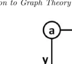
An edge is said to joinits two vertices. Likewise, two vertices are said to be adjacentif and only if there is an edge between them. Two vertices are said to beconnectedif there is a path from one to the other via any number of edges.
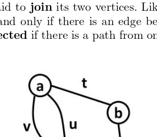
The example graph in Figure 2.1 has 5 labeled vertices and 7 labeled edges. Vertexais connected to every vertex in the graph, but it is only adjacent to vertices c andb. Note that edgesuand v, which can both be written (a, c), are multiple edges. Edgey, which can also be written (d, d) is a loop. Vertex
bhas degree 2 because 2 edges use it as an endpoint. Some kinds of edges are special.
Definition 2.3 Loop
Aloopis an edge that joins a vertex to itself.
Definition 2.4 Multiple Edge
In a graphG, an edge is amultiple edgeif there is another edge in E(G) which joins the same pair of vertices.
A multiple edge can be thought of as a copy of another edge—two line segments connecting the same two points.
Loops and multiple edges often make manipulating graphs difficult. Many proofs and algorithms in graph theory require them to be excluded.
Definition 2.5 Simple Graph
Asimple graphis a graph with no loops or multiple edges.
An edge always has exactly two vertices, but a single vertex can be an endpoint for zero, one, or many edges. This property is often very important when analyzing a graph.
Definition 2.6 Degree
In a graphG, thedegreeof a vertexv, denoteddegree(v), is the number of timesv occurs as an endpoint for the edgesE(G).
In other words, the degree of a vertex is the number of edges leading to it. However, loops are a special case. A loop adds 2 to the degree of a vertex since both of its endpoints are that same vertex. The degree of a vertex can also be thought of as the number of other vertices adjacent to it (with loops counting as 2).
2.3
Comparing Graphs
2.3.1
Subgraphs
Recall that a graph is simply defined as a set of vertices and edges. If we consider only a subset of those vertices and a subset of those edges, we are considering asubgraph. Asubgraphfits the definition of a graph, so it is in turn a graph (which may in turn have its own subgraphs).
Definition 2.7 Subgraph AsubgraphS of a graphGis:
• A set of verticesV(S)⊂V(G).
• A set of edges E(S)⊂E(G). Every edge in E(S) must be an unordered pair of vertices (v1, v2) such thatv1∈V(S) andv2∈V(S).
The last line of this definition tells us that an edge can only be part of a subgraph if both of its endpoints are also part of the subgraph.
2.3.2
Induced Subgraphs
The definition of a subgraph has two parts, but what if you were only given one of those parts and asked to make a subgraph? This is the notion of an
induced subgraph. Subgraphs can be induced in two ways: by vertices or by edges.
Definition 2.8 Induced Graph (Vertices)
In a graph G, the subgraph S induced by a set of vertices N ⊂ V(G) is composed of:
• V(S) =N
• For all pairs of verticesv1∈V(S) andv2∈V(S), if (v1, v2)∈E(G), then
(v1, v2)∈E(S).
You can think of a subgraph induced by a set of vertices like a puzzle. Given some set of verticesN ⊂V(G), find all the edges in Gwhose endpoints are both members ofN. These edges make up the edges of the induced subgraph. The darker part of the graph in Figure 2.2 is a subgraph of the whole. This subgraph is induced by the vertices{b, c, d} or by the edges{w, x}.
Subgraphs can also be induced by edges.
Definition 2.9 Induced Graph (Edges)
In a graph G, the subgraph S induced by a set of edges M ⊂ E(G) is composed of:
• E(S) =M
• For each edge (v1, v2)∈E(S),v1∈V(S) andv2∈V(S).
FIGURE 2.2: An induced subgraph.
M ∈ E(G), find all the vertices in V(G) that are endpoints of any edges in
M. These vertices make up the vertices of the induced subgraph.
2.3.3
Isomorphic Graphs
It is helpful to think of graphs as points connected by lines. This allows us to draw them and visualize the information they contain. But the same set of points and lines can be drawn in many different ways. Graphs that have the same structure have the same properties and can be used in the same way, but it may be hard to recognize that two graphs have the same structure when they are drawn differently.
Definition 2.10 Graph Isomorphism
Two graphs G and H are isomorphic(denoted G ≃ H) if there exists a bijection f such thatf :V(G)→V(H) such that an edge (v1, v2)∈E(G) if
and only if (f(v1), f(v2))∈E(H).
Informally, this means that two graphs are isomorphic if they can both be drawn in the same shape. IfG and H are isomorphic, the bijection f is said to be an isomorphismbetween Gand H and between H andG. The
isomorphism classofGis all the graphs isomorphic toG.
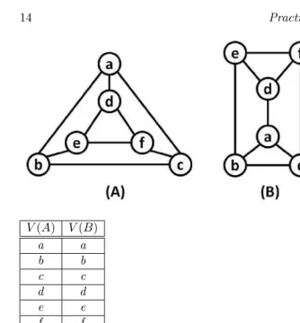
Figure 2.3 shows three graphs: A, B, and C. All three graphs are isomor-phic, but only A and B are automorphic. The first table shows one automor-phism between A and B. The second table shows the isomorautomor-phism between A and C.
2.3.4
Automorphic Graphs
V(A) V(B)
a a
b b
c c
d d
e e
f f
V(A) V(C)
a f
b b
c a
d c
e e
f d
FIGURE 2.3: An example isomorphism and automorphism.
Labeled graphs are isomorphic if their underlying unlabeled graphs are isomorphic. In other words, if you can remove the labels and draw them in the same shape, they are isomorphic. But what if you can draw them in the same shape with the same labels in the same positions? This is the notion of automorphicgraphs. Two automorphic graphs are considered to be the same graph.
Definition 2.11 Graph Automorphism
Anautomorphismbetween two graphsGandH is an isomorphismf that mapsGonto itself.
When an automorphism exists betweenGandH they are said to be au-tomorphic. The automorphism class of G is all graphs automorphic to
G.
at first, so more explanation is required. Both an isomorphism and an auto-morphism can be thought of as a function f. This function takes as input a vertex fromGand returns a vertex fromH. Now suppose thatGandH have both been drawn in the same shape. The functionf is an isomorphism if, for every vertex inG,f returns a vertex fromHthat is in the same position. The functionf is an automorphism if, for every vertex in G, f returns a vertex fromH that is in the same locationandhas the same label. Note that all au-tomorphisms are isomorphisms, but not all isomorphisms are auau-tomorphisms.
2.3.5
The Subgraph Isomorphism Problem
One common problem that is often encountered when mining graphs is the
subgraph isomorphism problem. It is phrased like so:
Definition 2.12 Subgraph Isomorphism Problem
Thesubgraph isomorphism problemasks if, given two graphsGandH, doesGcontain a subgraph isomorphic toH?
In other words, given a larger graphGand a smaller (or equal sized) graph
H, can you find a subgraph in Gthat is the same shape asH?
This problem is known to be NP-complete, meaning that it is computation-ally expensive. Algorithms that require us to solve the subgraph isomorphism problem will run slowly on large graphs—perhaps so slowly that it is not practical to wait for them to finish.
2.4
Directed Graphs
Edges have so far been defined as unordered pairs, but what if they were made into ordered pairs? This is the idea behind adirected graphordigraph. In these kinds of graphs, edges work one way only.
Definition 2.13 Directed Graph
A directed graphD is composed of two sets: a set of verticesV(D) and a set of edgesE(D) such that each edge is an ordered pair of vertices (t, h). The first vertext is called thetail, and the second vertexhis called thehead.
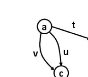
An edge in a directed graph is usually drawn as an arrow with the arrow-head pointing toward the arrow-head vertex. In a directed graph, you can follow an edge from the tail to the head butnot back again. Directed graphs require us to redefine some of the terms we established earlier.
FIGURE 2.4: An example directed graph.
Definition 2.14 Indegree
In a digraph D, theindegreeof a vertexv is the number of edges in E(D) which have vas the head.
Definition 2.15 Outdegree
In a digraphD, theoutdegreeof a vertexvis the number of edges inE(D) which have vas the tail.
Definition 2.16 Digraph Isomorphism
Two digraphsJ andKareisomorphicif and only if their underlying undi-rected graphs are isomorphic.
Note that, like labeled graphs, we ignore the direction of the edges when considering isomorphism. Two digraphs are isomorphic if you can change all the directed edges to undirected edges and then draw them in the same shape.
2.5
Families of Graphs
Some kinds of graphs that obey certain rules are known to have helpful proper-ties. We now discuss some common families of graphs that you will encounter in this book.
2.5.1
Cliques
Definition 2.17 Clique
A set of vertices C is a clique in the graph G if, for all pairs of vertices
v1∈Candv2∈C, there exists an edge (v1, v2)∈E(G).
If you begin at one vertex in a clique, you can get to any other member of that clique by following only one edge.
A clique is very similar to the idea of acomplete graph. In fact, a clique is exactly the same as a complete subgraph.
Definition 2.18 Complete Graph
Acomplete graphwithnvertices, denotedKn, is a graph such thatV(Kn)
is a clique.
A complete simple graph has all the edges it can possibly contain, but just how many edges is that? Consider the fact that every vertex is adjacent to every other vertex. That means each vertex in a complete graph with n
vertices will have degreen−1. To find the number of edges, we simply multiply the degree of each vertex by the number of vertices and divide by 2. We need to divide by 2 because each edge gets counted twice (since it connects two vertices). Thus, the total number of edges in a complete graph is n(n2−1).
In Figure 2.5, graph A contains a clique of size 5. If we remove vertex
f, graph A is a complete graph. Graph B shows a path of length 4 between verticesaande. Graph C shows a cycle of length 5.
2.5.2
Paths
If you think of the vertices of a graph as cities and the edges of a graph as roads between those cities, a path is just what it sounds like: a route from one city to another. Like a set of driving directions, it is a set of roads which you must follow in order to arrive at your destination. Obviously, the next step in a path is limited to the roads leading out of your current city.
Definition 2.19 Path (Edges)
A path of length n, denoted Pn, in a graph G is an ordered set of edges
{(v0, v1),(v1, v2),(v2, v3), . . . ,(vn−1, vn)} such that each edgee∈E(G).
A path can also be defined in terms of vertices, but the concept is the same.
Definition 2.20 Path (Vertices)
A path of length n, denoted Pn, in a graph G is a set of n + 1
ver-tices {v1, v2, . . . , vn, vn+1} such that for i from 1 to n, there exists an edge
(vi, vi+1)∈E(G).
A path is sometimes called awalk. Note that there may be more than one path between the same two vertices in a graph.
Now that we have defined a path, we can revisit an earlier concept from the beginning of this chapter and define it more precisely.
Definition 2.21 Connected Vertices
Two vertices are connected if and only if there exists a path from one to the other.
Definition 2.22 Connected Graph
A graph Gis a connected graph if, for every vertexv, there is a path to every other vertex in V(G).
In other words a connected graph cannot have any parts which are unreach-able, such as a vertex that is not an endpoint for any edge. In future chapters of this book, when we use the term graph, we mean a simple connected graphby default.
A path issimple if it never visits the same vertex twice. A path isopen
if its first and last vertices are different. A path is closedif its first and last vertices are the same.
2.5.3
Cycles
There is another name used to describe a closed path.
Definition 2.23 Cycle
Acycleof lengthn, denotedCn, in a graphGis a closed path of lengthn.
A simple cycleis the same as a simple closed path, with the exception that it may visit one vertex exactly twice: the vertex which is both the start and end of the cycle.
Note that, like Kn above, Pn and Cn name graphs (which may be
sub-graphs of other sub-graphs). If a graph contains a cycle of length 5, it is said to containC5.Pn, or the “path graph” can be drawn as a line.Cn, or the “cycle
2.5.4
Trees
Trees are graphs that obey certain structural rules and have many appealing mathematical properties. Like trees in nature, a treegraph has exactly one vertex called theroot. This root, orparent, can have any number ofchildren
vertices adjacent to it. Those children can, in turn, be parents of their own children vertices, and so on. A vertex which has no children is called aleaf.
Definition 2.24 Tree
A graphGis atreeif and only if there is exactly one simple path from each vertex to every other vertex.
Trees are sometimes defined in a different but equivalent way:
Definition 2.25 Tree
A graphGis atreeif and only if it is a connected graph with no cycles. The graph in Figure 2.6 is a tree, and vertexais the root. The root has 3 children:b,c, andd. Verticesd,e,f,h, andiare leaves. Vertexcis the parent ofg. Vertexais an ancestor ofg and, likewise, vertexg is the descendant of
a.
Trees are often modeled as directed graphs. If this is the case, the root vertex must have indegree 0. It will have outdegree equal to the number of its children. All vertices other than the root have indegree exactly 1. That one incoming edge must be coming from the parent vertex. Leaf vertices have outdegree 0.
Similar to a human family tree, we can define that vertex dis a descen-dantof vertexaif there is a path fromato d. All of a vertex’s children are its descendants, but not all of its descendants are its children; they might be its grandchildren or great grandchildren.
Likewise, we can define that vertex ais an ancestorof vertex dif there is a path fromatod. A vertex’s parent is its ancestor, but a vertex can have
ancestors which are not its parent (i.e., grandparents, great grandparents, etc.).
Note that trees are defined recursively. If you consider only a child vertex and all of its descendants as a subgraph, it is also a tree that has that vertex as the root.
2.6
Weighted Graphs
Many kinds of graphs have edges labeled with numbers, or weights. The weight of an edge often represents the cost of crossing that edge.
Definition 2.26 Weighted Graph
A weighted graphW is composed of two sets: a set of verticesV(W) and a set of edgesE(W) such that each edge is a pair of verticesv1 andv2 and a
numeric weight w.
Weighted graphs are often used in path-finding problems. Consider Fig-ure 2.7. There are many shortest paths from vertex a to vertex d, because there are many ways to reachdby only crossing 3 edges. The path{a, b, e, d}
and the path{a, c, e, d}are both shortest paths.
However, when we consider the cost of a path, there is only one lowest cost path. The path{a, b, e, d}costs 5 + 9 + 2 = 16. The path{a, b, e, d}only costs−3 + 15 + 2 = 14, so it is the lowest cost path.
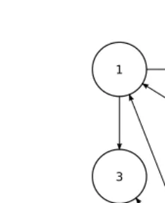
FIGURE 2.8: Two example graphs, an undirected version (A) and a directed version (B), each with its vertices and edges numbered.
2.7
Graph Representations
There are several different ways to represent a graph, each with its own ad-vantages and disadad-vantages. For each example, we will refer to the graphs in Figure 2.8. For the definitions below, letn=|V(G)|, the number of vertices in the graph. Letm=|E(G)|, the number of edges in the graph. In both graphs in Figure 2.8,n= 5 andm= 7.
2.7.1
Adjacency List
The adjacency list is the simplest and most compact way to represent a graph.
Definition 2.27 Adjacency List
Given a graph G such that V(G) = {v1, v2, . . . , vn}, the adjacency list
representation ofGis a list of lengthnsuch that theithelement of the list is
a list that contains one element for each vertex adjacent tovi.
The adjacency list for graph A is:
Graph A: [1] [2, 3, 3] [2] [1, 4] [3] [1, 1, 4] [4] [2, 3, 5] [5] [4, 5]
The adjacency list for graph B is:
[1] [2, 3, 3] [2] []
[3] [4] [4] [2, 5] [5] [5]
If you have the adjacency list of a graph, you can easily answer the ques-tion, “Which vertices are adjacent to theith vertex?” To find which vertices
are adjacent tov2in graph A, look at the second element of graph A’s
adja-cency list. It contains a list of the vertices that have edges leading to or from
v2. In this case, we see thatv2 is adjacent tov1 andv4.
This representation requires the least amount of memory to represent on a computer, so it is ideal for very fast algorithms. Specifically, an adjacency list requires about n+ 2m bytes for an undirected graph and about n+m
bytes for a directed graph. Algorithms exist for finding a path between two vertices that can run inO(n+m) time, so this representation would be ideal in that case.
2.7.2
Adjacency Matrix
An adjacency matrix is similar to an adjacency list.
Definition 2.28 Adjacency Matrix
Given a graphGsuch thatV(G) ={v1, v2, . . . , vn}, theadjacency matrix
representation ofGis an×nmatrix. Ifar,cis the value in the matrix at row
rand column c, thenar,c= 1 ifvris adjacent tovc; otherwise,ar,c= 0.
The adjacency matrix for graph A is:
The adjacency matrix for graph B is:
If you have the adjacency matrix of a graph, you can easily answer the question, “Arevr andvcadjacent?” To determine if there is an edge between
v2 andv4 in graph A, we can check the adjacency matrix for graph A at row
2, column 4. The value at that location is 1, so an edge does exist.
but many graph algorithms (like the ones discussed in this book) require Ω(n2)
time. In other words, the amount of time it takes to set up an adjacency matrix is not very much when compared to how long the algorithm will take to run.
2.7.3
Incidence Matrix
The incidence matrix representation is less popular than the adjacency matrix, but it can still be helpful in certain situations.
Definition 2.29 Incidence Matrix
The incidence matrix for graph A is:
The incidence matrix for graph B is:
If you have the incidence matrix of a graph, you can easily answer the question, “Which vertices make up an edge?” Consider edge e4 in graph B.
To find out which vertex is the tail, we can look through the 4th column on
the incidence matrix until we find the value −1 at row 3. This means that vertexv3 is the tail of edgee4. Likewise, we see that vertexv4 is the head of
FIGURE 2.9: Problems 1 and 2 refer to this graph.
2.8
Exercises
1. Count the number of the following in Figure 2.9:
(a) Vertices (b) Edges
(c) Multiple edges (d) Loops
(e) Vertices adjacent to vertexa
(f) Vertices connected to vertex a
2. Draw the subgraph induced by the following in Figure 2.9:
(a) Induced by the vertices{a, b, c, d, e}
(b) Induced by the edges{x, y, z}
FIGURE 2.10: Problem 3 refers to these graphs.
3. In Figure 2.10, are graphsY andZ isomorphic? If so, give an iso-morphism. Are they automorphic? If so, given an autoiso-morphism. 4. A planar graph is a graph that can be drawn on a plane (such as
(a) Draw a planar clique of size 4. (b) Draw a planar clique of size 5. (c) Draw a planar clique of size 6.
5. Draw an undirected tree and then attempt to do the following tasks. Conjecture which of these tasks are possible and which are impos-sible:
(a) Draw a directed tree with the same number of vertices and edges.
(b) Draw a new undirected tree with the same number of vertices but a different number of edges.
(c) Add an edge to the tree without creating a cycle.