A DISTANCE-WEIGHTED GRAPH-CUT METHOD FOR THE SEGMENTATION OF
LASER POINT CLOUDS
Avishek Dutta, Johannes Engels and Michael Hahn
Stuttgart University of Applied Sciences Schellingstr. 24
D-70174 Stuttgart, Germany [email protected]
Commission III,WG III/2
KEY WORDS:graph, cut, segmentation, laser point cloud
ABSTRACT:
Normalized Cut according to (Shi and Malik 2000) is a well-established divisive image segmentation method. Here we use Normalized Cut for the segmentation of laser point clouds in urban areas. In particular we propose an edge weight measure which takes local plane parameters, RGB values and eigenvalues of the covariance matrices of the local point distribution into account. Due to its target function, Normalized Cut favours cuts with “small cut lines / surfaces”, which appears to be a drawback for our application. We therefore modify the target function, weighting the similarity measures with distant-depending weights. We call the induced minimization problem“Distance-weighted Cut”(DWCut). The new target function leads to a slightly more complicated generalized eigenvalue problem than in case of the Normalized Cut; on the other hand, the new target function is easier to interpret and avoids the just-mentioned drawback. DWCut can be beneficially combined with an aggregation in order to reduce the computational effort and to avoid shortcomings due to insufficient plane parameters.
Finally we present examples for the successful application of the Distance-weighted Cut principle. The method was implemented as a plugin into the free and open source geographic information system SAGA; for preprocessing steps the proprietary SAGA-based LiDAR software LIS was applied.
1 INTRODUCTION
Segmentationdenotes the task of partitioning a set (e.g. the pix-els of an image or the points of a laser point cloud) into disjoint sets, whose elements share certain properties or exhibit similar-ities with respect to certain attributes. In the case of images, mostly low-level features like intensity, hue or vicinity are em-ployed as segmentation criteria; for laser point clouds also geo-metric attributes like local plane parameters, point densities etc. come into consideration.
There are roughly speaking two groups of segmentation methods, see e.g. (Gonzalez and Woods 2002): The first category is based onsimilarity. Starting with elements having locally extremal val-ues of a distinguishing attribute, elements with similar valval-ues are successivelyaggregatedby a region growing. The second cat-egory of methods is based ondiscontinuity. Abrupt changes in the criterion function are detected, often by evaluating gradients, in order to determine the borders between two adjacent subsets. While such borders are not necessarily closed curves / surfaces, the segmentation turns out to be much simpler if this holds true; any enclosed region can then be immediately associated with a segment. The requirement is automatically fulfilled for divisive algorithms, which subdivide the image / point cloud successively into smaller pieces.
2 NORMALIZED CUT - BASIC DEFINITIONS
Normalized Cut (Shi and Malik 2000) is an established divisive segmentation method. Its applications reach from low-level tasks like image compression to semantic interpretation, e.g. the in-terpretation of medical images, (Carballido-Gamio et al. 2004). While it was originally conceived for perceptual grouping in raster
images, it has been successfully applied for the segmentation of laser point clouds as well, see e.g. (Reitberger 2010). The ba-sic model ofNormalized Cutis an undirected weighted graph G = (V,E), featuring the elements of a setV, e.g. pixels or laser points, as nodes (vertices). Edenotes the set of edges, i.e. of all pairs of non-identical nodes(u, v), u, v∈V. To each edge (u, v)a non-negative “edge weight”w(u, v)is assigned which represents a similarity measure comparing the connected nodes
u, v. The graphGis successively subdivided into smaller sub-graphs: ”In grouping we seek to partition the set of vertices into disjoint setsV1,V2, . . .Vm, where by some measure the simi-larity among the vertices in a setViis high and, across different setsVi,Vjis low.” (Shi and Malik 2000). This is achieved by minimizing in each decomposition step a cost function, which is essentially determined by the edge weights of the cut edges.
The choice of the cost function is decisive for the segmentation result. Cost functions are expressed in terms of theassociationof two arbitrary setsA,B, which is defined by
assoc(A,B) :=X u∈A
X
v∈B
w(u, v) (1)
Nodes are serially numbered; we shall mostly write the weights in index notationWijinstead ofw(u, v)wherei, j∈ {1,2, . . . N} andNis the number of nodes inV. If we require the setsA,Bto be just two disjoint subsets whose union equals the setV,assoc itself represents a possible cost function, which is calledcutin this case:
cut(A,B) :=assoc(A,B) (2)
cuts where one of the resulting subsets is small:cut(A,B)tends to be small if the number of edges to be cut is small. For this reason, (Shi and Malik 2000) introduced a modified cut crite-rion, calledNormalized Cut, which avoids the disadvantages of the minimum cut criterion:
Ncut(A,B) := cut(A,B) assoc(A,V)+
cut(A,B)
assoc(B,V) (3)
The authors point out that ”the cut that partitions out small iso-lated points will no longer have smallNcutvalue, since the cut value will almost certainly be a large percentage of the total con-nection from that small set to all other nodes” (ibidem). That means, if e.g. the subsetAis small, not onlycut(A,B), but alsoassoc(A,V)will be small, so thatNcutwill not automati-cally assume small values. Compared to other cost functions the minimization of the Ncut criterion can be achieved with relatively low computational effort.
For a constructive mathematical formulation, the edge weights are collected in the weight matrixW:= [Wij];Wis symmetric. Furthermore a diagonal matrixDis defined according to
Dii= X
k∈V
Wik (4)
Dcontains for each node the sum of the weights of all incident edges; it is therefore calledtotal connection matrix. The matrix L:=D−Wis calledLaplace matrix.
The subdivision of the graph is conveniently expressed by an in-dicator vectorxof dimensionN. The i-th element ofxis 1 if nodeibelongs to subsetAand -1 if nodeibelongs toB. With the definition of a second type of indicator vectors
˜
y:= assoc(B,V) (1+x)− assoc(A,V) (1−x) (5) the following equalities are easily obtained:
˜ yT(D
−W) ˜y= 4assoc(A,B)assoc2(V,V) ˜
yTDy˜= 4assoc(A,V)assoc(B,V)assoc(V,V)
and therefore
˜
yT(D−W) ˜y ˜
yTDy˜ = Ncut(A,B) (6)
The given definition ofy, is slightly different from the one in˜ (Shi and Malik 2000), however leads to the same results. Unconstrained minimization of the ratio (6) yields the following generalized eigenvalue problem:
(D−W) ˜y=λD˜y (7)
The eigenvaluesλof (7) represent theNcutvalues of the decom-positions which originate from the corresponding eigenvectors as indicator vectors. Therefore it seems that the eigenvector corre-sponding to the smallest eigenvector of (7) represents the solu-tion of the minimizasolu-tion problem (6). The solusolu-tion of the original problem, however, has to fulfil some constraints:
1. A particular combination of they˜ishould vanish:
1TDy˜= 0 (8)
2. The elements ofxmay assume only values 1 or -1, there-fore according to the definition (5), the elements ofy˜are
also constrained:
˜
yi∈ {2assoc(B,V), −2assoc(A,V)} (9)
3. The setsA,Bshould not be empty, i.e. the elements ofx should not be all the same.
The total connection matrixDis assumed to be positive definite, otherwise there is at least one node with no incident non-zero edges and the graphGcannot be connected. Furthermore, the Laplace matrixD−Wcan be shown to be positive-semidefinite. The smallest eigenvalue of the system (7) isλ= 0and the cor-responding eigenvectory1˜ =1/√N. This eigenvector clearly corresponds to the (undesired) case that all nodes are associated to the same subset, which is to be avoided according to the third constraint. Therefore, rather the eigenvector of (7) corresponding to the second-smallest eigenvalue has to be used.
It is easy to show that the first constraint is automatically fulfilled by all other eigenvectors. On the other hand, solutions of (7) will in general not fulfill the second constraint. Therefore the mini-mization of theNcutaccording to (6) under the given constraints is not equivalent with the computation of the eigenvector which belongs to the second smallest eigenvalue of the system (7). This problem seems to be unsolved. (Shi and Malik 2000) proposed the following pragmatic approach: Compute the eigenvector of (7) corresponding to the second smallest eigenvalue. Select a thresholdtand associate the nodes withy˜i≤tto subsetAand the nodes withy˜i > tto subsetB. This approach seems to be sufficient and effective for all practical computations. Regarding the numerical solution, (Shi and Malik 2000) proposed to solve this transformed system by means of theLanczos method, see e.g. (Golub and Van Loan 2013).
3 EDGE WEIGHT FUNCTIONS FOR LASER POINT CLOUDS
(Shi and Malik 2000) give examples for the segmentation of im-ages. They use a weight function, which is a multiplicative com-bination of a distance-depending part and a part comparing the greyvalues of the pixels:
Wij= exp(−||
Fi−Fj||2
σ2 I
)∗
exp(−||Xi−Xj||2
σ2 X
) if||Xi−Xj||< r
0 otherwise
(10)
Here Fi, Fj denote the greyvalues of the pixelsi, j. σI, σX denote two scale factors,ra threshold for the consideration of the weightWij. Obviously the distance between two pixels directly effects their ”similarity”.
they are located on a common planar segment. By a plane fit-ting in a preprocessing step the point cloud may be augmented with local plane parameters as additional attributes. Of course such plane parameters are meaningless for line-like or spatially isotropic point distributions, e.g. along power lines or on a rough vegetation surface. For such cases the eigenvalues of the covari-ance matrices of the local point distributions represent valuable information about the type and the spatial extension of the regis-tered objects, upon which information a similarity measure may be based, see e.g. (Gross and Thoennessen 2006), (Jutzi and Gross 2009).
The experimental investigations for the present study were per-formed in the framework of the free and open-source geographic information system SAGA; for preprocessing steps the propri-etary SAGA-based LiDAR software LIS was used. SAGA / LIS provide modules for local plane-fitting, colour enrichment and for the eigenvalue computation of covariance matrices of local point distributions. If no colour information is available, intensity val-ues of the laser reflections may be used. In our proposal for a weight function for LiDAR point clouds we therefore assume that for each point of the point cloud either local plane parameters or eigenvalues of the local point distribution are available.
We propose the following weight function between two LiDAR pointsi,j: if both points have valid plane parameters
WDist
if none of the points has valid plane parameters
0 otherwise
(11) HerecP,c(1)RGB,c
(2)
RGB,cEare user-selected constant coefficients, the weight contributionsWm
ij, m ∈ {N, O, RGB, E}are ex-plained in the following. This weight function obviously implies that points with valid plane parameters and points without such parameters are always grouped into disjoint segments. The con-stant coefficients are normalized according to
cP+c(1)RGB= 1, c (2)
RGB+cE= 1 (12)
Those coefficients control the relative impact of the weight con-tributionsWN
ij ∗WijO,WijRGBorWijE,WijRGB, respectively. As all weight contributionsWm
ij, m ∈ {N, O, RGB, E}vary be-tween 0 and 1, the range ofWijis therefore also[0,1].
3–1 Distance-dependent Weight Contribution
For the distance-dependent weight contributionWDist ij we pro-pose an exponential decay similar as in (10):
WijDist:= we introduce a point-dependent scale factorc̺: The local point density of mobile laser data may vary considerably depending on the distance of the scanner to the targeted surface and the inci-dence angle of the laser rays. That means, these variations may
be characteristic for the measuring process rather than for the tar-geted object and do not necessarily correspond to properties of the material surface. If they are not compensated, theNormalized Cut principle favours cuts along surfaces where the local point density is low, because there are relatively few connections to be cut, so the correspondingcut(A,B)is relatively small.
3–2 Similarity Measures based on Plane Parameters, RGB values and Eigenvalues of the Covariance Matrix
The termsWN
ij,WijO in (11) are to quantify how well the plane parameters of the pointsi,jare compatible and how close each of the points is located to the local plane of the other point. We use the common implicit plane representation
<N,X>−d= 0 (14) whereNdenotes the unit normal vector of the plane anddits dis-tance of from the origin. The weight contributionWN
ij measures the similarity between the normal vectors of the pointsi,j:
WN
This measure is not sufficient for the comparison of planes, as parallel planes with an offset cannot be distinguished by (15). An analogous expression for the similarity of the distancedis not invariant against translational motions of the coordinate system. We therefore prefer to use the distances of a point from the best fitting plane of the other point instead:
WijO = exp
N, σO2 are global scale factors. The similarity contributions (15), (16) are not redundant. Simple geometric configurations can be cited for which one of these measures reaches its maximum while the other remains small. For a good coincidence of the two local planes we require high values for both criteria; therefore their contributions are combined in a multiplicative way.
For the comparison of the RGB values and the eigenvalues of the covariance matrices we propose simple Euclidean distances:
WRGB
i denote the greyvalues of pointiin the red, green and blue channel, λ(1)i , λ
(2) i ,λ
(3)
i the eigenvalues of the covariance matrix of the point distribution in the vicinity of point
i.σ2
RGB,σ2Eare global scale factors.
4 SEGMENTATION REQUIREMENTS AND
SHORTCOMINGS OF NORMALIZED CUT
TheNcutminimization condition together with the afore-mentioned weight function entails some implications, which may be consid-ered as drawbacks, depending on the particular application:
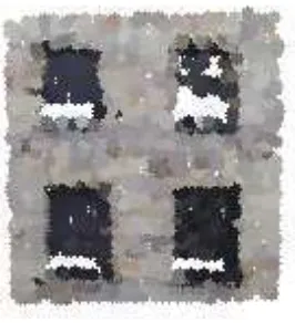
(a) RGB colour-enriched point cloud of a facade with windows
(b) Ncut segmentation of the point cloud. Colours indicate the segment affiliation of the points
Figure 1: Ncut of a facade
nodes, at the narrowest section there are relatively few edges or connections to be cut. This implies a relatively smallcut value, while the associationsassoc(A,V),assoc(B,V)in the denominator of (3) might be big, e.g. because there are a lot of connections among the members of one and the same subsetAorB. So the resultingNcutvalue tends to be small. For some applications the property seems to be adequate in-deed as e.g. for single tree detection from laser point clouds, see (Reitberger 2010). Here the distribution of the laser points in space essentially reflects the tree contours or sil-houettes. On the other hand, in the case of terrestrial laser point clouds the local point density is somewhat random and dependent on the distance to the scanner, and it will often be undesirable to cut slim-shaped point sets at their narrowest section as the subsets may anyway form a continuous object.
2. In a recursive application of the Normalized Cut, there may appear smallerNcutvalues on a deeper level of the recursion than on higher levels. If theNcutof the higher level exceeds the selected threshold, the smaller Ncuts in the deeper levels are never reached.
3. An addition of “remote” nodes, i.e. nodes which are far from the expected cut line or surface, may change theNcutvalue, as assoc(A,V), assoc(B,V) possibly change, whereas cut(A,B)may remain unaltered. The threshold for the ac-ceptance of a cut therefore appears arbitrary or at least hard to interpret.
For the purpose of segmentation of mobile laser scanning data, we encountered in particular the first implication as a severe draw-back. Figure (1) shows an example where the points of a building facade have been segmented by Normalized Cut. Obviously one of the windows is not “resolved”, on the other hand the facade is decomposed into several pieces; the borders between these pieces are mostly short lines, where only few connections had to be cut. See e.g. the upper border of the light green facade segment, which is short as it extends between two windows. This cut between the two windows is undesired, the more so as both resulting subsets exhibit very similar plane parameters and spectral properties. We propose therefore a modified minimization criterion, which avoids the afore-mentioned drawbacks.
5 DISTANCE-WEIGHTED CUT
5–1 Target Function of DWCut
As in (10) we assume again that the weightsWijare of the form
Wij=WijDistance·WijSimilarity, (18)
i.e. that they consist of a distance-dependent factor and a factor taking into account similarity measures like similarity of plane parameters, RGB values etc. In contrast to the foregoing sec-tions, here the term “similarity” does not include the distance be-tween the relevant nodes any more. Let us further assume that the graphGis totally connected with respect to the edge weight coefficientsWij.
We propose an alternative target function, which we call – in the same way as the corresponding minimization problem – the Distance-weighted Cut (DWCut):
DWCut(A,B) := cut(A,B)
cutD(A,B)
(19)
HerecutD(A,B)denotes the cut which results if only the distance-depending part of the weights is taken into account. Using (18), DWCutcan be written as
DWCut(A,B) := P i∈A
P j∈B
WDistance
ij ·W
Similarity ij
P i∈A
P j∈B
WDistance ij
(20)
DWCutcan be represented in terms of the indicator vectorx:
DWCut(A,B) = x T(D
−W)x xT(D
D−WD)x = x
TG˜x
xTH˜x (21)
whereWD,DDdenote the matrices of the coefficientsWijDistance,
DDistance
ij . Furthermore we use the abbreviationsG˜:=D−W, ˜
H :=DD−WD.
According to (20) the distance-weighted cut can be interpreted as a weighted average of the similarity measure over the cut edges ij, where the similarity measure is given byWSimilarity
ij and the
weight byWDistance
weights:
WijDistance=
( 1 if||X
i−Xj||< r 0 otherwise
) (22)
In this case,DWCutsimply equals the mean similarity measure over the cut edges (where only the edges with a length smaller thanrare taken into account).
It is easy to prove that the drawbacks of theNcut, which we have pointed out in section 4, are all avoided byDWCut. However, just like the solution ofNormalized Cut, the solution ofDWCutis not necessarily unique.
The distance-weighted cut has to be regularized, because oth-erwise its value would be undefined if all nodes are associated to the same set, i.e. if one of the setsA,B is empty. In this case the indicator vectorxisx = ±1, but(D−W)1 = 0, (DD−WD)1=0, so that both numerator and denominator of the target function (21) vanish.
Regularization of the denominator with a matrixRaccording to H:=DD−WD+Rleads to the modified minimization prob-lem
DWCut(A,B) =x TGx˜
xTHx !
= Minimum
under the constraints
a) xi∈ {1,−1} ∀i∈ {1. . . N}
b) The elements of x must not be all the same.
(23)
Neglecting constraint a), (23) leads to the following generalized eigenvalue problem:
˜
Gx= ˜λHx (24)
Two different regularization matrices suggest themselves:
a)R=x1xT1, withx1:=1/ √
N.
b)R=I.
It can be shown that for both regularizations the eigenvaluesλ˜k and eigenvectorsxk, k = 2. . . N of the problem (24) are not impaired, i.e.
Hxk= ˜Hxk (25)
5–2 Numerical Computation of the Distance-Weighted Cut
For the solution of the problem (23), we follow the approach of (Shi and Malik 2000) for the Normalized Cut: We initially ne-glect constraint a) of (23). As the smallest eigenvalue˜λ1of (23) corresponds to the eigenvectorx1=1/√N, i.e. to a decomposi-tion where all nodes go into one of the subsetsAorB, we search the eigenvector corresponding to the second smallest eigenvalue. Then we select a thresholdtand associate the nodes withxi≤t to subsetAand the nodes withxi> tto subsetB.
(24) is a slightly more complicated eigenvalue problem than (7), as the matrixHon the right hand side is not diagonal, in contrast to the matrixDin (7). Therefore a transformation to a standard eigenvalue problem requires a higher numerical effort.
It is in general easier to find the smallest eigenvector than the second smallest. Therefore we prefer toshiftthe eigenvalueλ˜1= 0to a higher value. This can be achieved by a modification of the matrixG˜ according to
G:= ˜G+x1xT1 (26)
It can be proved thatx1,xkwithk= 2. . . Nare also eigenvec-tors of the modified problem
Gx=λHx (27)
withλ1= 1, λk= ˜λk; instead of computing thesecond small-est eigenvalue of the system (24) and its corresponding eigenvec-tor, we may equivalently compute the smallest eigenvalue of the system (27) and its eigenvector.
For the solution of the system (27) or the computation of its eigenvector corresponding to the smallest eigenvalue, respectively, we apply a variant of theArnoldi algorithmwhich was proposed by (Golub and Ye 2002).
5–3 Preprocessing Steps
In a first step local plane parameters for all points of the point cloud are calculated. Then the distance weightsWDist
ij and the similarity weightsWijSimilarityare computed as described in sec-tion (3) and stored in a sparse matrix format. A convenient and efficient format is thecompressed-column representation(CCR) of a sparse matrix, see e.g. (Golub and Van Loan 2013) p. 598 ff.
When we introduced the target function of DWCut in section (5–1), we assumed that the graph is totally connected with re-spect to the distance-depending edge weightsWDist
ij , otherwise there were, apart fromx1, further eigenvectors of the generalized eigenvalue problem (24), for which the Rayleigh quotient in (23) was indeterminate. Therefore we have to decompose the graph into subgraphs that are totally connected. Each subgraph is rep-resented by a list of points; the list is initialized with an arbitrary point which has not been associated to a subgraph so far. Suc-cessively all neighboring points of the points in the list are added (with the term “neighboring point” here we denote a point, whose edge with the current point features a nonzero weight).
In the following step each subgraph is recursively subdivided by DWCutinto smaller segments, until the segments fall below a certain size or until the DWCut exceeds the selected threshold. The proposed solution method by (Golub and Ye 2002) yields local minima of the target function instead of the global mini-mum; the result may depend on the initial approximation of the indicator vector. It is therefore important to start from several initial approximations which have to be carefully selected. Ap-propriate approximations can be found by an algorithm similar to the one just described for the determination of subgraphs, while here a higher similarity than zero is required; the sets of nodes connected with this “minimal similarity” can be considered as approximate partitions.
6 A HYBRID SEGMENTATION METHOD: COMBINING DWCUT AND AGGREGATION
Figure 2: Blurred plane parameters cause insufficient partitioning (see text for explanation)
an arbitrary laser point, the neighbouring points within a sphere of a certain radius are selected; a plane is fitted to those points by an adjustment . As e.g. the spheres around the points B and C in the figure already contain points of the orthogonal connection be-tween the planes, the local normal vectors of the points B and C are deflected to the right. Accordingly the plane offset between B and C appears much smaller than the true valued, and therefore the decomposition of the point set fails: The plane parameters appear “blurred” across the edge of the protrusion, and the edge weight between the points B and C appears higher than it should be. Therefore a cut between B and C may be rejected.
This kind of blurring appears quite frequently and may seriously deteriorate the results of the segmentation; it is not a peculiar-ity ofDWCut, but may appear with other graph cut methods as well, if weight contributions of the form (15) and (16) are ap-plied. Since the drawback is rather due to the plane fitting than due to graph cut itself, it is hard to avoid without a preceding seg-mentation: If the affiliation of the points to planar segments is already known in the beginning, the plane fitting to an arbirtrary point could rely on the points within the same plane only. But the segmentation on its own is based on the plane parameters, so the snake bites its tail.
As a way out of this dilemma, we propose to compute the plane parameters as described, but perform a thinning of the point cloud before the subsequent segmentation. The thinning should be done in such a way, that in each voxel the point with the highest pla-narity is retained. In the following we call the retained points also “seed points”. In figure 2 most probably not the points B and C, but e.g. the points A and D would be retained, as the spheres around these points contain only neighbouring points which are situated on the related planes, therefore the planarity will be high and the plane parameters are not affected by “outliers”. Then the thinned point cloud is segmented byDWCut. The cut which separates the points A and D will probably be accepted, because the plane parameters of these two points are sufficiently differ-ent. Finally the residual points are aggregated to the seed points. As an aggregation criterion the similarity measures analogous to (16) and (17) can be used for the weight contributionsWO
ij,
WRGB
ij andWijE. However, in the case ofWijOwe recommend an asymmetric criterion: Only the plane parameters of the seed point should be taken into account, as the plane parameters of the residual point are not as reliable. That means,WO
ijis essentially based on the distance between the local seed point plane and the residual point. In this way also such points can be aggregated to a planar segment, which do not have valid plane parameters themselves.
The aggregation benefits from the preceding segmentation of the thinned point cloud: Without that segmentation a complicated merging procedure would be necessary, which was to combine
planar seed point segments with similar plane parameters. In the proposed workflow the merging is unnecessary, as the seed points themselves are already grouped by the segmentation. On the other hand, due to the preceding thinning, the segmentation proves to be easier and more reliable: Thanks to the relative high planarity of the points of the thinned point cloud the segmentation is more robust. Furthermore the computational effort ofDWCut is, by the reduction of the number of points, greatly reduced.
7 EXPERIMENTAL INVESTIGATIONS
As pointed out in section 3, we propose to define the similarity between two laser points with valid local plane parameters as a combined measure of the distances between the points in nor-mal vector space, RGB space and the mutual distances between one point and the local plane of the other point. The success of the algorithm is obviously dependent on how the parameters of the similarity function are defined; these parameters essentially control the decay of the similarity measure with increasing dis-agreement in one of the mentioned criteria and also the relative impact of the individual constituents. Furthermore the distance-dependent weight, which defines the relative impact of an edge similarity within the averaged cut, is of crucial importance. In general, choosing a relaxed value for a similarity criterion may group together semantically unrelated objects, while the choice of a strict value may produce undesired cuts. This trade-off is im-portant to realize and the choice of the parameters must be well guided by the nature of the application.
In the following we give some results of the Distance-weighted Cut algorithm, which also illustrate the influence of the similarity and weight parameters on the resulting segmentation.
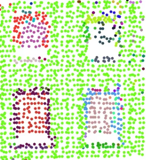
Figure 3: Segmentation result for the point cloud of figure 1 by DWCut
mostly do not as the embrasures are too narrow: the plane off-set between the facade and the window panes amounts to ca. 30 cm. Sometimes facade points and points on the window panes are very close to each other; this implies that the distinction be-tween the window segments and the facade segment is achieved by regular cuts and not by a separation of unconnected subgraphs. The cuts between facade and window panes were mostly effected by the constituentWO
ij in the similarity function. The example demonstrates that the proposed similarity function is appropriate to distinguish different planar segments. Although the “blurring” of the plane parameters as described in figure 2 actually appeared in the embrasures of the windows, for this example it did not af-fect the result, the more so as we selected a small neighbourhood radius in the computation of the local plane parameters. However, as we shall see, such blurring effects can not always be avoided. Very small segments (size< 5points) seldom signify anything of importance in the point cloud. We therefore applied a merg-ing algorithm as a post-processmerg-ing step in order to incorporate the small segments into bigger ones. The merging algorithm may choose to assign points of the small segments to bigger segments by checking which neighbouring segment’s local plane is closest to the point. If no neighbouring segment features a valid plane, the segment belonging to the closest neighbour wins the point. Figure 4 shows the result after the merging step.
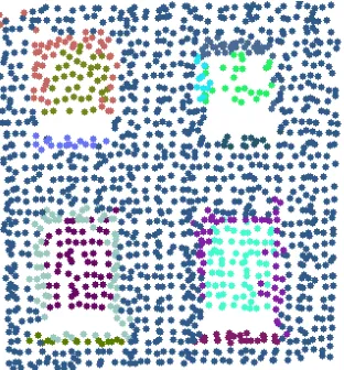
Figure 4: Segmentation result by DWCut for the point cloud of figure 3 after merging of small segments
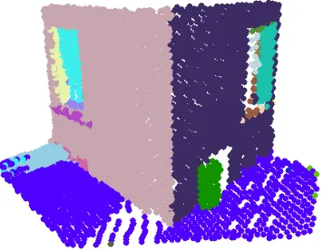
Figure 5: Colour-enriched point cloud containing a building edge
Figure 5 depicts a more complicated point cloud; most impor-tant objective is to see if the algorithms are able to reproduce the sharp building edge. Obviously with DWCut this failed as can be
Figure 6: Segmentation result for the point cloud of figure 5 with DWCut
seen in figure 6, region (4): Along the edge there are two (un-desired) elongated segments available. These segments appear since the local plane parameters, in particular the normal vectors, are “blurred” for the points near the edge. The neighbourhood of an arbitrary point close to the building edge may contain a consid-erable number of points of the adjacent facade, particularly if the chosen radius of the neighbourhood is relatively big. Therefore the edge is blurred in such a way that the normal vector is chang-ing gradually and this may give rise to additional segments. It might even occur that the plane fitting fails and the points do not feature valid plane parameters. These effects can be mitigated or even avoided, if for each point only a very small neighbourhood is employed for the computation of the plane parameters. The downside of this strategy is that the computed plane parameters are unreliable and unstable. This becomes apparent in region (1) of figure 6. Here the laser scan lines have a big distance to each other – bigger than the selected neighbourhood radius. There-fore the plane parameters in that region are mostly computed with points of one scan line at a time, which yields insignificant nor-mal vectors and therefore the apparent superfluous segment on the ground. The superfluous segment in region (3) of figure 6 is also for similar reasons.
Figure 7: Segmentation result for the point cloud of figure 5 with DWCut, tuned parameters
For our application, we wished to suppress the protrusion, so the segment in (2) was undesired. For this purpose we relaxed theσN2 parameter for the similarity of the normal vectors (0.08 to 0.75) and the correspondingσ2
dfor the distance-depending weight (0.8 to 1.2); the impact of the RGB similarity was reduced to 0 in or-der to avoid the effect of shadows etc. in the segmentation. In order to avoid the segments in (4) and to obtain a sharp build-ing edge, the plane parameters where computed from a smaller neighbourhood. Relaxing the distance parameterσd2 allows for a bigger neighbourhood, which is often helpful in bridging over wide scan lines.
Figure 7 shows the improved result. It is apparent that the pro-trusion segments have disappeared. As expected, the superfluous ground segments are still available. Also the problems on the building edge are still visible, though somewhat mitigated.
A considerable improvement is made by means of the hybrid algorithm according to section 6: The point cloud is thinned based on the best planarity among the points in a voxel. The thinned point cloud is segmented using DWCut and subsequently an aggregation is carried out, where the segmented points of the thinned point cloud act as seed points; each aggregated point in-herits the segment affiliation of the seed point to which it is ag-gregated.
Figure 8: Segmentation result for the point cloud of figure 5 with hybrid algorithm
Figure 8 shows the segmentation result of the hybrid algorithm. Here the undesired segments of the building edge have disap-peared; the edge is represented quite sharp. The ground is, apart from the stair at the left and some single points at the right, rep-resented by one segment. The big protrusion on the right face has been grouped into one segment, although it has two distinct planar facets. This is due to the fact, that the thinning procedure failed to locate a point with considerable planarity on the missing facet.
Finally, figure 9 shows the segmentation result by the hybrid method applied to the complete facade. Although some problems remain, the result confirms the potential of the proposed algorithms.
ACKNOWLEDGEMENTS
This work was funded by the German Federal Ministery of Ed-ucation and Research within the project “mms – Automatisierte Extraktion vertikaler Strukturen im st¨adtischen Bereich aus Mul-tisensor Mobile Mapping Daten”. The data used in this study was kindly provided by TopScan GmbH. Last not least, very helpful discussions with Volker Wichmann and Frederic Petrini of Laser-data GmbH, Innsbruck, Austria are gratefully acknowledged.
Figure 9: Segmentation result for a complete building facade with the hybrid algorithm
REFERENCES
Carballido-Gamio J, Belongie SJ, Majumdar S 2004: Normal-ized cuts in 3-D for spinal MRI segmentation. IEEE Trans Med Imaging January 2004 23(1): 36-44.
Gonzalez R and Woods R 2002: Digital Image Processing. 2nd Edition 2002. Prentice-Hall, Upper Saddle River, New Jersey.
Golub G and Van Loan Ch 2013: Matrix Computations. 4th Edi-tion 2013. John Hopkins University Press, Baltimore, Maryland.
Golub G and Ye Q 2002: An inverse free preconditioned Krylov subspace method for symmetric generalized eigenvalue prob-lems. SIAM Journal of Scientific Computing, Vol 24 Issue 1, pp 312-334
Gross H and Thoennessen U 2006: Extraction of Lines from Laser Point Clouds. In: W. F¨orstner and R. Steffen (eds), Pho-togrammetric Computer Vision, IAPRS, Vol. XXXVI Part3.
Jutzi B and Gross H 2009: Nearest Neighbor classification on Laser point clouds to gain object structures from buildings. IS-PRS Hannover Workshop 2009: High resolution earth Imag-ing for geospatial Information, Hannover, Germany. The Inter-national Archives of the Photogrammetry, Remote Sensing and Spatial Information Sciences , Vol. XXXVIII, Part 1-4-7/W5
Reitberger J 2010: 3D-Segmentierung von Einzelb¨aumen und Baumartenklassifikation aus Daten flugzeuggetragener Full Waveform Laserscanner. PhD Thesis Technische Universit¨at M¨unchen, Institut f¨ur Photogrammetrie und Fernerkundung
Shi J and Malik J 2000: Normalized Cuts and Image Segmenta-tion. IEEE Transactions on Pattern Analysis and Machine Intelli-gence, Vol. 22, No 8, pp 888-905, August 2000