A Model of Mortgage Default
JOHN Y. CAMPBELL and JO ˜AO F. COCCO∗
ABSTRACT
In this paper, we solve a dynamic model of households’ mortgage decisions incorpo-rating labor income, house price, inflation, and interest rate risk. Using a zero-profit condition for mortgage lenders, we solve for equilibrium mortgage rates given bor-rower characteristics and optimal decisions. The model quantifies the effects of ad-justable versus fixed mortgage rates, loan-to-value ratios, and mortgage affordability measures on mortgage premia and default. Mortgage selection by heterogeneous bor-rowers helps explain the higher default rates on adjustable-rate mortgages during the recent U.S. housing downturn, and the variation in mortgage premia with the level of interest rates.
THE EARLY YEARS OF THE 21ST CENTURY were characterized by unprecedented instability in house prices and mortgage market conditions, both in the United States and globally. After the housing credit boom in the mid-2000s, the housing downturn of the late 2000s saw dramatic increases in mortgage defaults. Fore-closures appear to have had negative feedback effects on the values of neigh-boring properties, worsening the decline in house prices (Campbell, Giglio, and Pathak (2011)). Losses to mortgage lenders stressed the financial system and contributed to the larger economic downturn. These events have underscored the importance of understanding household incentives to default on mortgages, and the way in which these incentives vary across different types of mortgage contracts.
In this paper, we study the mortgage default decision using a theoretical model of a rational utility-maximizing household. We solve a dynamic model of a household that finances the purchase of a house with a mortgage, and must in each period decide how much to consume and whether to exercise options to default, prepay, or refinance the loan. Several sources of risk affect household
∗John Y. Campbell is at the Department of Economics, Harvard University, and NBER, and Jo ˜ao F. Cocco is at the Department of Finance, London Business School, CEPR, CFS, and Netspar. We would like to thank seminar participants at the AEA 2012 meetings, Bank of England, Berkeley, Bocconi, Essec, the 2012 SIFR Conference on Real Estate and Mortgage Finance, the 2011 Spring HULM Conference, Illinois, London Business School, Mannheim, the Federal Reserve Bank of Minneapolis, Norges Bank, and the Rodney L. White Center for Financial Research at the Whar-ton School, as well as Stefano Corradin, Andra Ghent, Francisco Gomes, Jonathan Heathcote, John Heaton, Pat Kehoe, Ellen McGrattan, Steve LeRoy, Jim Poterba, Nikolai Roussanov, Sam Schulhofer-Wohl, Roine Vestman, Paul Willen, and Albert Zevelev for helpful comments on an earlier version of this paper. We are particularly grateful to three anonymous referees and to Ken Singleton (Editor) for comments that have significantly improved the paper.
DOI: 10.1111/jofi.12252
decisions and the value of the options on the mortgage, including house prices, labor income, inflation, and real interest rates. We use multiple data sources to parameterize these risks.
Importantly, we study household decisions for endogenously determined mortgage rates. We model the cash flows of mortgage providers, including a loss on the value of the house in the event the household defaults. We then use risk-adjusted discount rates and a zero-profit condition to determine the mort-gage premia that in equilibrium should apply to each contract. Since household mortgage decisions depend on interest rates and mortgage premia, and these decisions affect the profits of banks, we must solve several iterations of our model for each mortgage contract to find a fixed point. Thus, our model is not only a model of mortgage default, but also a micro-founded model of the determination of mortgage premia.
The literature on mortgage default emphasizes the role of house prices and home equity accumulation for the default decision. Deng, Quigley, and Van Order (2000) estimate a model, based on option theory, in which a household’s option to default is exercised if the option is in the money by some specific amount. Borrowers do not default as soon as home equity becomes negative; they prefer to wait since default is irreversible and house prices may increase. Earlier empirical papers by Vandell (1978) and Campbell and Dietrich (1983) also emphasize the importance of home equity for the default decision.
As in this literature, in our model mortgage default is triggered by negative home equity, which tends to occur for a particular combination of the shocks that the household faces: house price declines in a low-inflation environment with large nominal mortgage balances outstanding. Also as in previous litera-ture, households do not default as soon as home equity becomes negative.
A novel prediction of our model is that the level of negative home equity that triggers default depends on the extent to which households are borrowing constrained. As house prices decline, households with tightly binding borrowing constraints will default sooner than unconstrained households, because they value the immediate budget relief from default more highly relative to the longer-term costs. The degree to which borrowing constraints bind depends on the realizations of income shocks, the endogenously chosen level of savings, the level of interest rates, and the terms of the mortgage contract. For example, adjustable-rate mortgages (ARMs) tend to default when interest rates increase, because high interest rates increase required mortgage payments on ARMs, tightening borrowing constraints and triggering defaults.
We use our model to illustrate these triggers for mortgage default and to explore several interesting questions about the effects of the mortgage system on defaults and mortgage premia.
when interest rates are high—because high rates increase the required pay-ments on ARMs—whereas the reverse is true for FRMs.
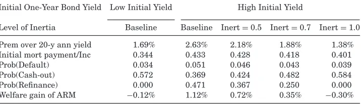
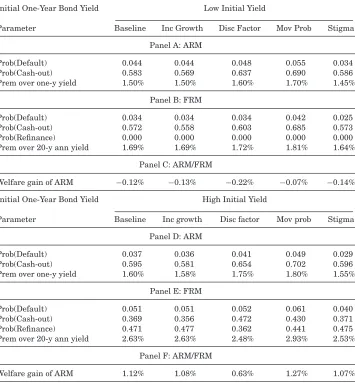
Second, we determine mortgage premia in the model and compare the results to the data. For most parameterizations and household characteristics the model predicts that mortgage premia should increase with the level of interest rates. In U.S. data, this appears to be the case for FRMs, but not for ARMs. The model is able to generate ARM premia that decrease with interest rates when we assume that ARM borrowers have labor income that is not only riskier on average, but also correlated with the level of interest rates. Such a correlation arises naturally if interest rates tend to be lower in recessions. We use our model to perform welfare calculations and show that households with this type of income risk benefit more from ARMs relative to FRMs, supporting the hypothesis that such households disproportionately borrow at adjustable rates. Even though our model can generate the qualitative patterns of mortgage premia observed in the data, it is harder to match those patterns quantitatively. Our model does not easily explain the large ARM premia observed in U.S. data when interest rates are low. Furthermore, our model generally predicts a larger positive effect of interest rates on FRM mortgage premia than that observed in U.S. data. Our model can deliver FRM mortgage premia that better match the data if there is refinancing inertia (Miles (2004), Campbell (2006)), so that households do not refinance their FRMs as soon as it is optimal to do so.1
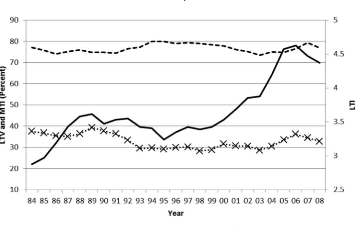
Third, we use our model to investigate how ratios at mortgage origination such as loan-to-value (LTV), loan-to-income (LTI), and mortgage-payment-to-income (MTI) affect default probabilities. The LTV ratio measures the house-hold’s initial equity stake, while LTI and MTI are measures of initial mortgage affordability. A clear understanding of the relation between these ratios and mortgage defaults is particularly important in light of the recent U.S. experi-ence. Figure1plots aggregate ratios for newly originated U.S. mortgages over the last couple of decades, using data from the Monthly Interest Rate Survey (MIRS) of mortgage lenders conducted by the Federal Housing Finance Agency (FHFA).2 This figure shows that there was an increase in the average LTV in
the years before the crisis, but to a level that does not seem high by historical standards. A caveat is that the survey omits information on second mortgages, which became far more common during the 2000s.3Even looking only at first
mortgages, however, there is a striking increase in the average LTI ratio, from an average of 3.3 during the 1980s and 1990s to as high as 4.5 in the mid-2000s. This pattern in the LTI ratio is not confined to the United States; in the United Kingdom the average LTI ratio increased from roughly two in the 1970s and 1980s to above 3.5 in the years leading up to the credit crunch (Financial Services Authority (2009)). Interestingly, as can be seen from Figure 1, the
1Guiso and Sodini (2013) provide a survey of the household finance literature.
2The LTV series is taken directly from the survey, and the LTI series is calculated as the ratio
of the average loan amount obtained from the same survey to the median U.S. household income obtained from census data. The survey is available atwww.fhfa.gov.
3In addition, the figure shows the average LTV, not the right tail of the distribution of LTVs,
Figure 1. LTV, MTI, and LTI over time for the United States.LTV data are from the MIRS of the FHFA, LTI are calculated as the ratio of the average loan amount obtained from the same survey to the median U.S. household income obtained from Census data, MTI are calculated using the same income measure and the loan amount, maturity, and mortgage interest rate data from the MIRS.
low interest rate environment in the 2000s prevented the increase in LTI from driving up MTI to any great extent.
Our model allows us to understand the channels through which LTV and initial mortgage affordability ratios affect mortgage default. A higher LTV ratio (equivalently, smaller down payment) increases the probability of negative home equity and mortgage default, an effect that is documented empirically by Schwartz and Torous (2003) and more recently by Mayer, Pence, and Sherlund (2009). The unconditional default probabilities predicted by our model become particularly large for LTV ratios in excess of 90%.
The LTI ratio affects default probabilities through a different channel. A higher initial LTI ratio does not increase the probability of negative equity; however, it reduces mortgage affordability, making borrowing constraints more likely to bind. The level of negative home equity that triggers default becomes less negative, and in turn default probabilities increase. Our model implies that mortgage providers and regulators should think about combinations of LTV and LTI rather than try to control these parameters in isolation.4
4Regulators in many countries, including Austria, Poland, China, and Hong Kong, ban high
Fourth, we model heterogeneity in labor income growth, labor income risk, and other household characteristics such as intertemporal preferences and in-herent reluctance to default. For instance, we consider two households that have the same current income, but differ in terms of the expected growth rate of their labor income. The higher the growth rate, the smaller are the in-centives to save, which increases default probabilities. However, we find that this effect is slightly weaker than the direct effect of higher future income on mortgage affordability, as measured, for example, by the MTI ratio later in the life of the loan. Therefore, the mortgage default rate and the equi-librium mortgage premium decrease with the expected growth rate of labor income.
Finally, we use our model to simulate developments during a downturn like the one experienced by the United States in the late 2000s. One motivation for this exercise is that, during the downturn, U.S. default rates were con-siderably higher for ARMs than for FRMs even though interest rates were declining, which contradicts our model’s prediction that ARMs default primar-ily when interest rates increase. To try to understand this fact, we simulate our model for a path of aggregate variables that matches the recent U.S. ex-perience of declining house prices and low interest rates. We show that one explanation for the higher default rates of ARMs is that ARMs are particu-larly attractive to households that face higher labor income risk, particuparticu-larly if their labor income is correlated with interest rates. In addition, we model ARMs with a teaser rate to capture the fact that interest-only and other al-ternative mortgage products have had higher delinquency and default rates than traditional principal-repayment mortgages (Mayer, Pence, and Sherlund (2009)).
Several recent empirical papers study mortgage default. Foote, Gerardi, and
Willen (2008) examine homeowners in Massachusetts who had negative home
equity during the early 1990s and find that fewer than 10% of these owners eventually lost their home to foreclosure, so that not all households with neg-ative home equity default. Bajari, Chu, and Park (2008) study empirically the relative importance of the various drivers behind subprime borrowers’ decision to default. They emphasize the nationwide decrease in home prices as the main driver of default, but also find that the increase in borrowers with high MTI ratios has contributed to increased default rates in the subprime market. Mian and Sufi (2009) further emphasize the importance of an increase in mortgage supply in the mid-2000s, driven by securitization that created moral hazard among mortgage originators.
The contribution of our paper is to propose a dynamic and unified microeco-nomic model of rational consumption and mortgage default in the presence of house price, labor income, and interest rate risk. Our goal is not to try to derive
the optimal mortgage contract (as in Piskorski and Tchistyi (2010,2011)), but instead to study the determinants of the default decision within an empirically parameterized model, and to compare outcomes across different types of mort-gages. In this respect, our paper is related to the literature on mortgage choice (see, for example, Brueckner (1994), Stanton and Wallace (1998,1999), Camp-bell and Cocco (2003), Koijen, Van Hermert, and Van Nieuwerburgh (2009), and Ghent (2013)). Our work is also related to the literature on the benefits of homeownership, since default is a decision to abandon homeownership and move to rental housing. For example, we find that the ability of homeowner-ship to hedge fluctuations in housing costs (Sinai and Souleles (2005)) plays an important role in deterring default. Similarly, the tax deductibility of mortgage interest not only creates an incentive to buy housing (Glaeser and Shapiro (2003), Poterba and Sinai,2011), but also reduces the incentive to default on a mortgage. Relative to Campbell and Cocco (2003), in addition to characteriz-ing default decisions, we make two main contributions. First, we assume that household permanent income shocks are only imperfectly correlated with house price shocks. This assumption is important since it allows us to assess, for each contract, the relative contributions of idiosyncratic and aggregate shocks to the default decision. Second, we use the profits of mortgage providers together with a zero-profit condition to solve for the mortgage premium that should apply to each contract.
Our paper is related to interesting recent research by Corbae and Quintin
(2015). They solve an equilibrium model to evaluate the extent to which
low down payment mortgages were responsible for the increase in foreclo-sures in the late 2000s, and find that mortgages with these features ac-count for 60% of the observed foreclosure increase. Garriga and Schlagen-hauf (2009) also solve an equilibrium model of long-term mortgage choice to examine how leverage affects the default decision, while Corradin (2014) solves a continuous-time model of household leverage and default in which the agent optimally chooses the down payment on an FRM, abstracting from inflation and real interest rate risk. Our paper does not attempt to solve for the housing market equilibrium, and therefore can examine household risks and mortgage terms in more realistic detail, distinguishing the contributions of short- and long-term risks, and idiosyncratic and aggregate shocks, to both the default decision and mortgage premia. We emphasize the influence of re-alized and expected inflation on the default decision, a phenomenon that is absent in real models of mortgage default. In this respect, our work comple-ments the research of Piazzesi and Schneider (2012) on inflation and asset prices.
The paper is organized as follows. In SectionI, we set up the model, build-ing on Campbell and Cocco (2003). This section also describes our solution
method and the calibration of model parameters. In Section II, we study
SectionIIIlooks at default rates conditional on specific realizations of aggre-gate state variables, thereby clarifying the relative contributions of aggreaggre-gate and idiosyncratic shocks to the default decision. A particular path that we study is one of declining house prices and low interest rates, which matches the recent U.S. experience. Section IVconcludes. An Internet Appendix pro-vides additional analysis.5
I. The Model
A. Setup
A.1. Time Parameters and Preferences
We model the consumption and default choices of a household i with a T -period horizon that uses a mortgage to finance the purchase of a house of fixed size Hi. We assume that household preferences are separable in housing and
nondurable consumption, and are given by
maxE1
where T is the terminal age,βi is the time discount factor,Cit is nondurable
consumption, and γi is the coefficient of relative risk aversion. The
house-hold derives utility from both consumption and terminal real wealth,Wi,T+1, which can be interpreted as the remaining lifetime utility from reaching age T +1 with wealthWi,T+1. Terminal wealth includes both financial and hous-ing wealth. The parameter bi measures the relative importance of the utility
derived from terminal wealth. Households are heterogeneous and our notation uses the subscriptito take this into account. We solve the model for different household characteristics.
Since we assume that housing and nondurable consumption are separable and that Hi is fixed, we do not need to include housing explicitly in household
preferences. However, the above preferences are consistent with
maxE1
forHit=Hi fixed, where the parameterθi measures the importance of housing
relative to nondurable consumption.
In reality Hi is not fixed and depends on household preferences and income,
among other factors. We simplify the analysis here by abstracting from housing choice, but we do study mortgage default for different values of Hi. In the
Internet Appendix, we consider a simple model of housing choice to assure that our main results are robust to this consideration.
5The latest Internet Appendix is available in the online version of the article on theJournal of
A.2. Interest and Inflation Rates
Nominal interest rates are variable over time. This variability comes from movements in both the expected inflation rate and the ex ante real interest rate. We use a simple model that captures variability in both these components of the short-term nominal interest rate.
We write the nominal price level at time t as Pt, and normalize the initial
price level to P1=1. We adopt the convention that lowercase letters denote log variables, and thus pt≡log(Pt) and the log inflation rate isπt= pt+1−pt.
To simplify the model, we abstract from one-period uncertainty in realized inflation; thus, expected inflation at time t is the same as inflation realized fromttot+1. While clearly counterfactual, this assumption should have little effect on our results since short-term inflation uncertainty is quite modest. We assume that expected inflation follows an AR(1) process. That is,
πt=µπ(1−φπ)+φππt−1+ǫt, (3)
whereǫtis a normally distributed white noise shock with mean zero and
vari-ance σǫ2. The ex ante real interest rate also follows an AR(1) process. The expected log real return on a one-period bond,r1t=log(1+R1t), is given by
r1t=µr(1−φr)+φrr1,t−1+εt, (4)
whereεtis a normally distributed white noise shock with mean zero and
vari-anceσε2.
The log nominal yield on a one-period nominal bond, y1t=log(1+Y1t), is
equal to the log real return on a one-period bond plus expected inflation:
y1t=r1t+πt. (5)
We let expected inflation be correlated with the ex ante real interest rate and denote the coefficient of correlation byρπ,r.
A.3. Labor Income and Taxation
Householdiis endowed with stochastic gross real labor income in each period t,Lit,which cannot be traded or used as collateral for a loan. As usual we use
a lowercase letter to denote the natural log of the variable, solit≡log(Lit). The
household’s log real labor income is exogenous and given by
lit= fi(t,Zit)+vit+ωit, (6)
where fi(t,Zit) is a deterministic function of agetand other individual
charac-teristicsZit, andvitandωitare random shocks. In particular,vitis a permanent
shock assumed to follow a random walk,
vit=vi,t−1+ηit, (7)
whereηitis an i.i.d. normally distributed random variable with mean zero and
i.i.d. normal distribution with mean zero and variance σω2i. Thus, log income is the sum of a deterministic component and two random components, one transitory and one persistent.
We let real transitory labor income shocks,ωit, be correlated with innovations
to the stochastic process for expected inflation,ǫt, and denote the corresponding
coefficient of correlation ρωi,ǫ. In a world where wages are set in real terms,
this correlation is likely to be zero. If wages are set in nominal terms, however, the correlation between real labor income and inflation may be negative. As before, we use the subscript i throughout to model the fact that households are heterogenous in the characteristics of their labor income, including the variance of the income shocks they face.
We model the tax code in the simplest possible way, assuming a linear taxa-tion rule. Gross labor income,Lit, and nominal interest earned are taxed at the
constant tax rateτ. We allow for deductibility of nominal mortgage interest at the same rate.
A.4. House Prices and Other Housing Parameters
We model house price variation as an aggregate process. Let PH
t denote the
date t real price of housing, and let pH
t ≡log(PtH). We normalize P1H=1 so thatHalso denotes the value of the house that the household purchases at the initial date. The real price of housing is a random walk with drift, so real house price growth can be written as
ptH=g+δt, (8)
wheregis a constant andδis an i.i.d. normally distributed random shock with mean zero and varianceσδ2. We assume that the shockδtis uncorrelated with
inflation, so in our model housing is a real asset and an inflation hedge. It would be straightforward to relax this assumption.
We assume that innovations to the permanent component of the household’s real labor income, ηit, are correlated with innovations to real house prices,
δt, and denote by ρηi,δ the corresponding coefficient of correlation. When this
correlation is positive, states of the world with high house prices are also likely to have high permanent labor income. We let innovations to the real interest rate be correlated with house price shocks, and denote this correlation byρε,δ.
We assume that in each period homeowners must pay property taxes, at rate τp, proportional to house value, and that property tax costs are income-tax
deductible. In addition, homeowners must pay a maintenance cost,mp,
A.5. Mortgage Contracts
The household is not allowed to borrow against future labor income. Fur-thermore, the maximum loan amount is equal to the value of the house less a down payment. The initial loan amount (Di1) is thus
Di1≤(1−di)P1P1HHi, (9)
wheredi is the required down payment. We use a subscription the required
down payment to allow for the possibility that it differs across households. We simplify the model by assuming that the household finances the initial
purchase of the house of size Hi with previously accumulated savings and
a nominal mortgage loan equal to the maximum allowed, (1−di)Hi. (Recall
that we normalize P1H and P1 to one.) The LTV and LTI ratios at mortgage origination are therefore given by
whereLi1denotes the level of household labor income at the initial date. Required mortgage payments depend on the type of mortgage. We consider several types, including FRMs, ARMs, and ARMs with a teaser rate.
LetYTi,F RM be the interest rate that householdi pays on an FRM with ma-turity T. It is equal to the expected interest rate over the life of the loan, or the yield on a long-term bond, plus an interest rate premium that depends on loan and borrower characteristics. The datetreal mortgage payment, MF RM
it ,
is given by the standard annuity formula:
MF RM
A distinctive feature of the U.S. mortgage market is that FRMs come with a refinancing option, which we model. In particular, if households take out FRMs when interest rates are high and rates subsequently decline, then households that have the required level of positive home equity, di, may refinance the
loan to take advantage of the lower interest rates. We assume that refinancing costs are equal to a proportion cr of the loan amount. We also assume that
households refinance into an FRM with remaining maturityT −tr+1, where
trdenotes the refinancing period. More specifically, we assume that households
refinance into the contract and the borrowing position that they would have been in periodtr had the interest rates at the time that the loan began been
lower.6
6This simplifies the numerical solution of the problem since we only need to solve the model
Let Y1i,tARM be the one-period nominal interest rate on an ARM taken out by householdi, and letDitARMbe the nominal principal amount outstanding at datet. The datetreal mortgage payment, MitARM, is given by
MitARM= Y
i,ARM
1t DitARM+DiARM,t+1 Pt
, (13)
whereDiARM,t+1 is the component of the mortgage payment at datetthat goes to pay down principal rather than pay interest. We assume that, for the ARM, the principal loan repayments,DARM
i,t+1, equal those for the FRM. This assumption simplifies the solution of the model since the outstanding mortgage balance is not a state variable.
The datetnominal interest rate for the ARM is equal to the short rate plus a constant premium
Y1i,tARM=Y1t+ψi,ARM, (14)
where the mortgage premiumψi,ARM compensates the lender for the prepay-ment and default risk of borroweri. In the case of an ARM with a teaser rate, the mortgage premium is set to zero for one initial period.
For an FRM the interest rate is fixed and equals the average interest rate over the loan maturity (the average zero-coupon bond yield for that maturity under the expectations hypothesis of the term structure) plus a premium ψi,F RM.
In addition to prepayment and default risk, the FRM premium compensates the lender for the interest rate refinancing option that borrowers receive. At times when the one-year yield is low (high), the term structure is upward (downward) sloping, and long-term rates are higher (lower) than short-term rates. As previously noted, we assume that mortgage interest payments are deductible at the income tax rateτ.
A.6. Mortgage Default and Home Rental
In each period, the household decides whether to default on the mortgage loan. The household may be forced to default because it has insufficient cash to meet the mortgage payment. However, the household may also find it optimal to default even if it has the cash to meet the payment.
We assume that, in the case of default, a mortgage lender has no recourse to the household’s financial savings or future labor income. The mortgage lender seizes the house, the household is excluded from credit markets, and since it cannot borrow the funds needed to buy another house it is forced into the rental market for the remainder of the time horizon. These assumptions sim-plify a complex reality. In the United States, the rules regarding recourse vary across states. In some states home mortgages are explicitly nonrecourse, whereas in others recourse is allowed but onerous restrictions on deficiency
judgments render many loans effectively nonrecourse.7In addition, defaulting
households in the United States are excluded from credit markets for a period of time but not permanently. To understand the effect of recourse, in the Inter-net Appendix we consider a variation of our model in which lenders can seize borrowers’ current financial assets in the event of default, but have no claim on their future labor income.
The rental cost of housing equals the user cost of housing times the value of the house (Poterba (1984), Diaz and Luengo-Prado (2008)). That is, the datet real rental costUitfor a house of sizeHi is given by
Uit=[Y1t−Et[exp(ptH+1+πt)−1]+τp+mp]PtHHi, (15)
where Y1t is the one-period nominal interest rate, Et[exp(ptH+1+π1t)−1] is
the expected one-period proportional nominal change in the house price, and τpandmpare the property tax rate and maintenance costs, respectively.8This
formula implies that in our model the rent-to-price ratio varies with the level of interest rates.9
Relative to owning, renting is costly for two main reasons. First, homeown-ers benefit from the income-tax deductibility of mortgage interest and property taxes, without having to pay income tax on the implicit rent they receive from their home occupancy. Second, owning provides insurance against future fluc-tuations in rents and house prices (Sinai and Souleles (2005)). When perma-nent income shocks are positively correlated with house price shocks, however, households have an economic hedge against rent and house price fluctuations even if they are not homeowners.
We assume that in the case of default the household is guaranteed a lower bound of Xin per-period cash-on-hand, which can be viewed as a subsistence level. This assumption can be motivated by the existence of social welfare pro-grams such as means-tested income support. In terms of our model, it implies that consumption and default decisions are not driven by the probability of extremely high marginal utility, which would be the case for power utility if there was a positive probability of extremely small consumption.
A.7. Early Mortgage Termination and Home Equity Extraction
We model several potential sources of early mortgage termination. As previ-ously mentioned, we allow FRM borrowers to take advantage of a decrease in
7Ghent and Kudlyak (2011) use variation in state laws to empirically evaluate the impact of
recourse on default decisions. Li, White, and Zhu (2011) argue that U.S. bankruptcy reform in 2005 affected mortgage default by making it harder for homeowners to use bankruptcy to reduce unsecured debt. See also the evidence in Demyanyk, Koijen, and Hemert (2010), and Chatterjee and Eyigungor (2009) and Mitman (2012), who solve equilibrium models of the macroeconomic effects of bankruptcy laws and foreclosure policies.
8To simplify we assume that maintenance costs are similar for homeowners and for rental
properties. Alternatively, we could have reasonably assumed that homeowners take better care of the properties, thereby reducing maintenance expenses.
interest rates by refinancing their mortgage. In addition, we allow households that have accumulated positive home equity to sell their house, repay the out-standing debt, and move into rental accommodation. The house sale is subject to a realtor’s commission, a fraction cof the current value of the property. In this way, at a costc, households are able to access their accumulated housing equity and use it to finance nondurable consumption. We interpret this event as a cash-out prepayment.10
Ideally, in addition to a cash-out prepayment, we would like to explicitly model other ways in which households can draw down their accumulated home equity, for example, using second mortgages or home equity lines of credit. Home equity extraction can play an important role in consumption smoothing and can have macroeconomic implications (Chen, Michaux, and Roussanov (2013)). Unfortunately, this would increase the already large number of state variables in our model, so we leave this topic for future research.
In addition to the above endogenous sources of mortgage termination, we model exogenous random mortgage termination by assuming that, in each period, with probabilityϕitborrowers are forced to move, in which case they sell
the house, repay the principal outstanding, and move into the rental market. If a household is hit with a moving shock at a time of negative home equity, the household defaults on the loan. We allow for the possibility that negative home equity creates a “lock-in” effect by letting the probability of a forced move be a lower valueϕit′ when home equity is negative.
A.8. Financial Institutions
We assume a competitive market for mortgage providers. In addition, we assume that financial institutions are able to screen borrowers and learn their characteristics. Therefore, the mortgage premium that they require for each contract will in equilibrium reflect the probability of prepayment, the default probability, and the expected losses given default of the specific borrower.11
LetC Fi jt(St) denote the dollar nominal cash flow that the lender receives from
householdion loan type jin periodtwhen the state isSt, for j= ARM,F RM.
By state Stwe mean a given combination of values for the state variables in
our model. Ex ante, many different values are possible; ex post, only one of them will be realized. The cash flow that lenders receive depends on whether householdichooses to default or prepay in periodt, given stateSt, if he or she
has not done so before. Given no default or prepayment, the lender receives the nominal mortgage payment
C Fi jt=PtMitj,forDde fi jtC =DCprepayi jt =0, (16)
10In this paper, we use the terms cash-out, cash-out prepayment, and cash-out refinancing
interchangeably.
11Since default and prepayment decisions depend on interest rates and mortgage premia, which
where DC
de fi jt (DCprepayi jt) is an indicator variable for default (prepayment) by
householdiin periodt. When default occurs, the lender loses the outstanding mortgage principal but receives the house. We assume that foreclosure involves a deadweight cost equal to a proportion loss of the value of the house. The nominal cash flow received by the mortgage lender is given by
C Fi jt=(1−loss)PtPtHHi,for Dde fi jtC =1. (17)
In the case of early mortgage termination due to a cash-out, the mortgage lender receives the outstanding loan principal,
C Fi jt =Ditj,forD C
prepayi jt =1. (18)
For the FRM there may also be early termination due to interest rate refi-nancing, in which case the lender receives the outstanding loan principal plus the refinancing cost paid by the borrower,
C Fi,F RM,t=DitF RM+cr(1−di)Hi,forDre fi jtC =1, (19)
whereDC
re fi jtis an indicator variable for refinancing by householdion mortgage
type j in period t. In periods subsequent to early mortgage termination or default, the nominal cash flows received by the lender are zero. This assumes that, in the case of FRM interest rate refinancing, borrowers take out a loan with a different mortgage provider.
We calculate the present value of the cash flows that the mortgage lender receives by discounting them using a risk-adjusted discount rate. We describe the pricing kernel in the Internet Appendix. Let PV1[C Fi jt](S1,S2, . . . ,St)
de-note the present value (at the initial date) of the period t cash flow for loan type j taken out by householdi. This present value depends not only on the value of the datetstate variables, but also on the value of the state variables in previous periods since they affect the rate that is appropriate for discounting the profits.12 We scale the present value of the sum of the cash flows by the
loan amount to calculate risk-adjusted profitability,
P Ri j(S)= T
t=1PV1[C Fi jt](S1,S2, . . . ,St)
(1−di)Hi
, (20)
whereS=[S1,S2, . . . ,ST]. This gives us a measure of the return on each loan
type, j=ARM,F RM, for a given borrower typeiand a given realization of the state variables. If at the initial date we take expectations across all possible realizations of the state variables,
P Ri j(S1)=E1[P Ri j(S)], (21)
12Only a subset of the state variables will affect the discount rate, namely, the aggregate
we obtain a measure of expected profitability of mortgage loan type j to bor-rower type i conditional on the values of the state variables at the time the mortgage is taken out.
These profitability calculations do not subtract administrative expenses and should be interpreted accordingly. Computationally it would be straightforward to subtract expenses when calculating the profits of mortgage providers, but one would need to specify the type of expenses (per period or up front, fixed or as a proportion of the loan value).
B. Model Summary and Solution
B.1. Model Summary
The state variables of the household’s problem are age (t), cash-on-hand (Xit), whether the household has previously terminated the mortgage through
prepayment or default (DS
termi jt, equal to one given a previous prepayment or
default and zero otherwise), real house prices (PH
t ), the nominal price level
(Pt), inflation (πt), the real interest rate (r1t), and the level of permanent
in-come (vit). For the FRM there is an additional state variable, namely, whether
the household has previously refinanced the loan (Dre fi jtS , equal to one given a previous refinancing and zero otherwise).
The choice variables are consumption (Cit), whether to default on the
mort-gage loan if no default has occurred before (DCde fi jt, equal to one if householdi chooses to default on loan jin periodtand zero otherwise), and in the case of positive home equity whether to prepay (DC
prepayi jt, equal to one if the household
chooses to prepay the mortgage in periodtand zero otherwise). For the FRM, there is an additional choice variable, namely, whether to refinance the loan (DC
re fi jt, equal to one if householdichooses to refinance the mortgage in period
tand zero otherwise).
In all periods before the last, if the household has not defaulted on or termi-nated its mortgage, its cash-on-hand evolves as follows for the case of an ARM:
Xij,t+1=(Xit−Cit)
for j=ARM. Savings earn interest that is taxed at rateτ. Next period’s cash-on-hand is equal to savings plus after-tax interest, minus real mortgage pay-ments (made at the end of the period), minus property taxes and maintenance expenses, plus next period’s labor income and the tax deduction on both nomi-nal mortgage interest and property taxes.
amount equal to the difference between the loan amount on the new loan and the amount outstanding on the refinanced loan.13
If the household has defaulted on or prepaid its mortgage and moved to rental housing, the evolution of cash-on-hand is given by
XiRent,t+1=(Xit−Cit)
(1+Y1t(1−τ))
(1+πt)
−Uit+Li,t+1(1−τ), (23)
whereUitdenotes the datetreal rental payment.
Terminal, that is, dateT +1, wealth is given by
Wij,T+1 = PT+1Xi,T+1+PT+1P
If the household has not previously defaulted or terminated the mortgage con-tract, terminal wealth is equal to financial wealth plus housing wealth. In the rental state, households only have financial wealth at the terminal date.
Households derive utility from real terminal wealth, so that in all of the above cases nominal terminal wealth is divided by a composite price index, denoted by PTComposite+1 . This index is given by
PTComposite+1 =
where (recall that)γi is the coefficient of relative risk aversion andθimeasures
the preference for housing relative to other goods in the preference specifica-tion(2). The above composite price index is consistent with our assumptions regarding preferences (Piazzesi, Schneider, and Tuzel (2007)). The fact that nominal terminal wealth is scaled by a price index that depends on the price of housing implies that, even in the penultimate period, homeownership serves as an hedge against house price fluctuations (Sinai and Souleles (2005)). The larger isθi, the stronger is such a hedging motive for homeownership.
B.2. Solution Technique
Our model cannot be solved analytically. The numerical techniques that we use for solving it are standard. Since the mortgage premium depends on mort-gage type, borrower characteristics, and the initial values of the aggregate state
13The speed at which FRM principal is repaid depends on the initial interest rate. We take this
variables, we solve the model separately for each of these cases. Recall that we normalize the initial price level and house prices to one, so that, as far as the aggregate variables are concerned, we need to calculate the mortgage premium for different initial levels of the inflation rate and the real interest rate.
The expected risk-adjusted profitability of each mortgage contract depends on the mortgage premium, which affects the default and prepayment decisions of borrowers, which in turn affect the expected risk-adjusted profitability of the loan. Therefore, for each case, we need to solve several iterations of our model to find a fixed point. We do so using a grid for mortgage premia with steps of five basis points. We start by making a guess for the mortgage premium, and then solve the borrower’s problem given that premium. Once we have the borrower’s optimal decisions, we use the transition probabilities and pricing kernel to calculate expected risk-adjusted profitability. We then iterate: if the expected risk-adjusted profitability is too high (low), we decrease (increase) the mortgage premium and solve the household’s problem again.
For each possible mortgage premium, we solve the borrower’s problem by discretizing the state space and using backwards induction starting from period T +1. The shocks are approximated using Gaussian quadrature, assuming two possible outcomes for each of them. This simplifies the numerical solution of the problem since for each periodtwe only need to keep track of the number of past high (low) inflation shocks, high (low) permanent income shocks, and high (low) house price shocks to determine the datetprice level, permanent income, and house prices. For each combination of the state variables, we optimize with respect to the choice variables. We use cubic spline or, in the areas in which there is less curvature in the value function, linear interpolation to evaluate the value function for outcomes that do not lie on the grid for the state variables. In addition, we use a log scale for cash-on-hand. This ensures that there are more grid points at lower levels of cash-on-hand.
To handle the refinancing option for FRMs, we solve the model sequentially, starting with the lowest level of initial interest rates, and save the value func-tion. We then use this value function in each periodtsubsequent to mortgage origination as an input for the borrower’s refinancing decision in the solution for the case of higher initial interest rates.
C. Parameterization
C.1. Time and Preference Parameters
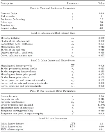
Table I
Baseline Parameters This table reports the parameter values used in the baseline case.
Description Parameter Value
Panel A: Time and Preference Parameters
Discount factor β 0.98
Risk aversion γ 2
Preference for housing θ 0.3
Initial age 20
Terminal age 50
Bequest motive b 400
Panel B: Inflation and Real Interest Rate
Mean log inflation µπ 0.029
St. dev. of the inflation rate σǫ 0.009
Log inflation AR(1) coefficient φπ 0.891
Mean log real rate µr 0.012
St. dev. of the real rate σr 0.018
Log real rate AR(1) coefficient φr 0.825
Correl. inflation and real rate ρπ,r 0.597
Panel C: Labor Income and House Prices
Mean log real income growth lt 0.008
St. dev. permanent income shocks ση 0.063
St. dev. temporary income shocks σω 0.225
Mean log real house price growth g 0.003
St. dev. house price return σδ 0.162
Correl. perm. inc. and house price shocks ρη,δ 0.191
Correl. real int. rate and house price shocks ρε,δ 0.300
Correl. temp. inc. and inflation shocks ρω,ǫ 0.000
Panel D: Tax Rates and Other Parameters
Income tax rate τ 0.25
Property tax rate τp 0.015
Property maintenance mp 0.025
Lower bound on cash-on-hand X $1,000
Transaction costs of house sale cs 0.060
Exogenous moving probability ϕ 0.040
Exogenous mov. prob. if negative equity ϕ′ 0.008
Panel E: Loan Parameters
Initial loan to income LT I 4.5
Initial loan to value LT V 0.90
FRM refinancing cost cr 0.01
importance of terminal wealth,b, is set to 400. This value is large enough to ensure that households have an incentive to save, and that our model generates
reasonable values for wealth accumulation. Panel A of Table I summarizes
C.2. Interest and Inflation Rates
We use data from the Livingston survey of inflation expectations to param-eterize the stochastic process for expected inflation (median one-year forecast, sample period 1987 to 2012). We obtain information on one-year nominal bond yields from the Federal Reserve and calculate the expected one-year real in-terest rate by deflating the nominal yield by expected inflation. The estimated parameters for the AR(1) processes for the logarithm of expected inflation and the logarithm of the expected real rate are reported in Panel B of TableI. The implied half-life of expected inflation shocks is six years, while the half-life for real interest rate shocks is 3.6 years.
C.3. Labor Income
We use data from the Panel Study of Income Dynamics (PSID) for the years 1970 to 2005 to calibrate the labor income process. Our income measure is broadly defined to include total reported labor income plus unemployment com-pensation, workers comcom-pensation, Social Security transfers, and other trans-fers for both the head of the household and his spouse. We use such a broad measure to implicitly allow for the several ways in which households insure themselves against risks of labor income that is more narrowly defined. Labor income is deflated using the Consumer Price Index.
It is widely documented that an individual’s income profile varies with ed-ucational attainment (see, for example, Gourinchas and Parker (2002)). To control for this relation, we follow existing literature and partition the sample into three education groups based on the educational attainment of the head of the household. For each education group we regress the log of real labor income on age dummies, controlling for demographic characteristics such as marital status and household size, and allowing for household fixed effects. We use this smoothed income profile to calculate, for each education group, the average household income for age 30 and the average annual growth rate in household income for ages 30 to 50. The estimated real labor income growth rate for households with a high-school degree is 0.8%, and we use this value in the benchmark case. The assumption of a constant income growth rate is a simplification of the true income profile that makes it easier to carry out comparative statics and investigate the role of future income prospects on the default decision.
C.4. House Prices
To calibrate the parameters of the house price process, also reported in Panel C of Table I, we use PSID data and Case-Shiller house price indices. The advantage of PSID data is that they contain both house price and labor income information. However, annual data, which we need to calculate annual house price returns, are only available until 1997. Furthermore, PSID house prices are self-reported and vulnerable to measurement error.
Using PSID household-level data, we obtain real house prices by dividing self-reported house prices by the consumer price index, and we calculate changes in house prices as the first difference of log real house prices for individuals who are present in consecutive annual interviews and who report not having moved since the previous year. To address potential measurement error, and parallel to our treatment of labor income, we winsorize the logarithm of real house price changes at the 5thand 95thpercentiles (−36.6% and 40.3%, respectively). We use the winsorized data to calculate the expected value and the standard deviation of real house price changes, which are equal to 1.6% and 16.2%, respectively (as before we also consider alternative parameterizations). Next we estimate the correlation between labor income shocks and house price shocks. To do so we first calculate
(lit− ˆfit)=[lit− ˆf(t,Zit)]−[li,t−1− ˆf(t−1,Zi,t−1)]=ηit+ωit−ωi,t−1,
(27)
where ˆf denotes the predicted regression values. The correlation between(27)
and the first differences in log house prices, δt, is positive and statistically
significant, and equal to 0.037. Under the model assumption that tempo-rary labor income shocks,ωit, are serially uncorrelated and uncorrelated with
house price shocks, this value implies a correlation between permanent labor income shocks, ηit, and house price shocks, δt, equal to 0.191. This value
re-flects the fact that a significant component of the innovations to permanent labor income shocks is idiosyncratic (and therefore uncorrelated with house prices).
We also use the S&P/Case-Shiller 10-City Composite Home Price Index to parameterize the model. The sample period is 1987 to 2012. We are particularly interested in the relation between house prices and real interest rates. As before, we deflate the house price index by the Consumer Price Index and calculate the logarithm of annual real house price growth. The mean log real house price growth, 0.005, is higher than that estimated in the PSID data due to the differences in the period covered. The standard deviation of log real house price growth, 0.09, is somewhat lower than in the PSID data. We estimate a positive correlation between innovations to the logarithm of real interest rates and log real house price returns equal to 0.38, with a p-value of 0.07. We parameterize the model using a somewhat lower value of 0.30. We set the remaining model correlations to zero.14
14We have estimated the correlation between log real house price returns and expected inflation,
The S&P/Case-Shiller composite house price index is less volatile than self-reported house prices from the PSID, because idiosyncratic house price variation diversifies away in the composite index.15Our model abstracts from
idiosyncratic house price variation. Nonetheless, we calibrate it using an estimate of total house price volatility since all movements in house prices, not just aggregate movements, affect homeowners’ incentives to default on their mortgages.
C.5. Tax Rates and Other Parameters
We follow Himmelberg, Mayer, and Sinai (2005) in setting the values for the tax rates. More specifically, we set the income tax rate, τ, equal to 0.25, the property tax rate,τp, equal to 0.015, and property maintenance expenses,mp,
equal to 0.025. In addition, we assume that a house sale is subject to a realtor commission,tc, equal to 6% of the value of the house, which is a fairly standard
value. We set the lower bound on (real) cash-on-hand to $1,000. We set the exogenous probability of a house move for borrowers with positive home equity
to 0.04. Chan (2001) estimates that an increase in LTV to over 95% would
result in a moving probability that is 20% of the original. Therefore, in the case of negative home equity we set the exogenous moving probability to 0.008. We report these parameters in Panel D of TableI.
C.6. Loan Parameters
We consider alternative values for the down payment/initial LTV and LTI, but to facilitate discussion we refer to the case in which the LTV ratio is 0.9 and the LTI is 4.5 as the baseline. We set the costs of refinancing the FRM contract tr to 1% of the loan amount. The credit risk premium on each of the mortgage
loans,ψi j, wherei denotes the borrower and j=F RM,ARM,is determined endogenously. We report the baseline loan parameters in Panel E of TableI.
D. Simulated Data
We solve the model separately for each mortgage type, set of borrower char-acteristics, and combination of initial values for the aggregate variables. Since we normalize the initial price level and real house prices to one, the aggre-gate variables we need to consider are expected inflation and the real interest rate. In the numerical solution we assume two possible states for each of these, which implies four different values for the initial one-year nominal rates. For each case, once we find a fixed point for the problem, we use the optimal policy functions to generate simulated data.
Agents in our model are subject to both aggregate and idiosyncratic shocks. Aggregate shocks are to real house prices, the inflation rate, and real interest
15This diversification effect is also visible in data on median U.S. house prices from the Monthly
rates. Idiosyncratic shocks are innovations to the permanent component of the labor income process (which also have an aggregate component since labor income is positively correlated with house price shocks) and temporary labor income shocks.
We first generate one realization for the aggregate shocks. Next, for this realization of aggregate shocks, we generate realizations for the shocks to the labor income process for 50 individuals. We then use the model policy functions, the one path for the aggregate variables, and the individual income shocks to simulate optimal consumption, prepayment, refinancing, and default behavior for these 50 individuals. We repeat this process for 800 paths for the aggregate variables, and for 50 individuals for each of these paths, which yields for each initial value of the aggregate variables, mortgage type, and borrower type a total of 40,000 different paths. We use the same realizations for the shocks to simulate consumption and default behavior for each of the different mortgage types that we study.
To understand the basic properties of the simulated data, in the Internet Appendix we plot the age profiles of cross-sectional average real gross income, consumption, and cash-on-hand. Real consumption is on average considerably lower than real gross income. The reason is that part of gross income must be paid in taxes, and the individual must also make mortgage payments and other housing-related expenditures such as property taxes and maintenance expenses. Part of income is also saved.16
In the next section, we use the simulated data to predict unconditional de-fault, prepayment, and refinancing probabilities. These probabilities, calcu-lated across the different paths for the aggregate and idiosyncratic variables in the model, are expected probabilities calculated at the initial date. Ex post, only one of the many possible paths for the aggregate variables will be realized. SectionIIIstudies probabilities conditional on a specific path. This analysis al-lows us to determine the relative contributions of aggregate and idiosyncratic shocks to default. Of particular interest is a path of low interest rates and declining house prices, which replicates the economic conditions that followed the recent U.S. crisis.
II. Unconditional Default Rates
A. Mortgage Default Triggers for ARMs and FRMs
We are interested in determining what triggers default in our model. We focus our attention on home equity and the MTI ratio. The empirical literature on mortgage default emphasizes the importance of home equity for the default
16Although not completely visible in the figure provided in the Internet Appendix, there is a
decision (see, for example, Deng, Quigley, and Van Order (2000), or more re-cently Foote, Gerardi, and Willen (2008), and Bajari, Chu, and Park (2008)).
To measure home equity, we calculate for each householdiand each datet the current debt outstanding as a fraction of current house value
LT Vi jt=
Di jt
PtPtHHit
, (28)
whereDi jtdenotes the loan principal amount outstanding on mortgage jat date
t, Pt the price level, andPtHthe real price of housing. An LT Vi jt greater than
one corresponds to negative home equity. Equation (28)shows that negative home equity tends to occur for a particular combination of the state variables: house prices are declining, the price level is low, and there are large mortgage balances outstanding (i.e., early in the life of the loan).17
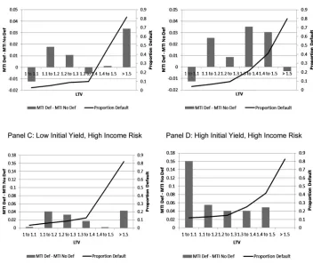
In Figure2we plot default probabilities for ARMs conditional on the level of negative equity. These probabilities are shown as solid lines in four alternative cases. In panels A and B we plot the results for the baseline level of income risk (a standard deviation of temporary income shocks of 0.225), and in Panels C and D we plot results for a higher level of income risk (a standard deviation of 0.35). Further, Panels A and C show the results for a low initial interest rate (defined as the lowest interest rate in our discretization of the model), while Panels B and D show the results for a high initial interest rate (defined as the second-highest discrete interest rate, since the highest rate is extreme and rarely observed). We use these two levels of interest rates throughout our presentation of results to illustrate the properties of the model.
The default probabilities in Figure 2 are calculated using one observation per mortgage, so that, for those households that choose never to default, even in the face of negative equity, we calculate these probabilities using the lowest level of equity that the household observes over the life of the mortgage. This approach is similar to that used by Bhutta, Dokko, and Shan (2010), who study default rates for nonprime borrowers from Arizona, California, Florida, and Nevada.
Figure2 shows that few households default at low levels of negative home equity. For most of the cases considered, the probability of default is less than 10% for LTVs up to 1.3. Thus, households only exercise their option to default when it is considerably in the money. This prediction of our model is consistent
with Bhutta, Dokko, and Shan (2010), who find that the median homeowner
does not default until equity falls to−62% of their home’s value, and with Foote, Gerardi, and Willen (2008), who study 100,000 homeowners in Massachusetts who had negative equity during the early 1990s and find that fewer than 10% of these owners lost their home to foreclosure.
17In our model the probability of negative equity first rises, as negative shocks have time to
Figure 2. Difference in MTI between households that default and households that do not default and the proportion of defaults as a function of home equity for the ARM contract.The data are obtained by simulating the model for the ARM contract. Low (high) income risk refers to households with a standard deviation of temporary income shocks equal to 0.225 (0.35). LTV is the ratio of current house value to the outstanding loan principal. The vertical bars plot, for each level of negative home equity, MTI for those households that choose to default minus MTI for those households that choose not to default.
The prediction that borrowers do not default as soon as home equity becomes negative is a prediction of all default models based on real option theory. A special feature of our model is that the MTI ratio also plays an important role:
MT Ii jt =
Mi jt
Lit
. (29)
At the most basic level this is illustrated by the fact that ARM default rates are higher for borrowers with high labor income risk who take out ARMs at high initial rates (Panel D of Figure2).
choose not to default. Focusing first on the case of low income risk, at very low levels of negative home equity the few borrowers who default do so because they are forced to move. This explains the fairly small (and even slightly negative) differences in MTI between the two groups of borrowers. When home equity becomes more negative and initial interest rates are high (Panel B), the MTI ratio becomes more important for the default decision. Its importance is most visible in Panel D, where the combination of high initial rates and high income risk leads households to endogenously default at relatively low levels of nega-tive home equity, and where there are large differences in current MTI between defaulting and nondefaulting borrowers. Large MTI, in the presence of borrow-ing constraints and low savborrow-ings, forces a choice between severe consumption cutbacks and mortgage default. Elul et al. (2010) provide empirical evidence of the importance of liquidity considerations for mortgage default decisions.
The default probabilities in Figure 2 show that, at high levels of negative home equity, the vast majority of borrowers decide to default. At these levels, wealth motives tend to be an important determinant of default decisions. This is consistent with the empirical findings of Haughwout, Okah, and Tracy (2014). They study mortgage redefault using data on subprime mortgage modifications for borrowers who were seriously delinquent and whose monthly mortgage pay-ment was reduced as part of the modification. They find that the redefault rate declines relatively more when the payment reduction is achieved through prin-cipal forgiveness as compared to lower interest rates. The empirical analysis of Doviak and MacDonald (2012) also emphasizes the role of modifications that reduce loan balances in preventing default.18
To better understand the importance of wealth and cash-flow motives for mortgage decisions, Table IIreports the means of several variables for ARM borrowers who choose to default, for borrowers with negative home equity but who choose not to default, for borrowers who choose to cash out, and for borrowers who take no action (regardless of whether they have negative home equity). In contrast with Figure2, in this table each household-date pair is an observation, so any given mortgage is observed multiple times and possibly in multiple states.
As before, we report results for low and high initial interest rates, and for low and high income risk. Across these four cases, we see that households with negative home equity that default tend to have more negative home eq-uity than those with negative home eqeq-uity but who choose not to default. In addition, households that choose to default are those with lower income and larger MTI. The larger MTIs are also the result of higher nominal interest rates. The difference in MTIs is larger when initial interest rates and income risk are high: in this case the average MTI is equal to 0.40 for households that default compared to an average MTI ratio of 0.34 for households with negative equity that choose not to default. TableIIalso reports the difference between mortgage and rent payments scaled by household income. For households sig-nificantly underwater that choose to default, doing so allows for a reduction in
The
Journal
of
Finance
R
Risk, and Conditional on Initial Interest Rates
This table reports the mean for several variables for the ARM contract by household action (default, no default given negative home equity, cash-out, no action). The table reports means across aggregate states and individual shocks, conditional on the initial level of interest rates. Low (High) initial rate corresponds to the state with the lowest (second-highest) level of interest rates in our model. The top (bottom) panels report results for the case in which the standard deviation of income shocks is equal to 0.225 (0.35). For each case the first column reports means for observations in which individuals choose to default, the second column reports means for observations in which individuals have negative home equity but choose not to default, the third column reports means for observations in which individuals choose to cash out, and the last column reports means for observations in which individuals choose neither to default nor to cash out (in case they have not done so before). Current LTV is the loan-to-value at the time of the action (or no action). In the means reported, each observation corresponds to an individual and time period. The probabilities of default and cash-out prepayment are the proportion of households who choose to default or cash out over the life of the mortgage.
Panel A: Low Initial Rate, Low Income Risk Panel B: High Initial Rate, Low Income Risk
Def No def|Eq<0 Cash-out No act Def No def|Eq<0 Cash-out No act
Current LTV 1.43 1.11 0.42 0.55 1.41 1.15 0.43 0.54
Price level 1.17 1.08 1.29 1.26 1.23 1.17 1.35 1.32
Real house price 0.45 0.69 1.34 1.08 0.45 0.59 1.32 1.07
Real income 46.6 47.7 48.8 52.5 46.3 48.0 48.5 52.6
Real cons t−1 13.9 15.1 13.4 14.9 13.4 14.2 12.9 14.5
Mort/Inc 0.33 0.29 0.31 0.28 0.33 0.33 0.33 0.30
(Mort-Rent)/Inc 0.26 0.22 0.05 0.12 0.26 0.24 0.05 0.11
Nom int rate 0.037 0.022 0.041 0.037 0.039 0.038 0.047 0.044
Age 36.4 33.2 39.3 38.3 36.4 34.6 39.0 38.3
Probability 0.044 0.583 0.037 0.595
Panel C: Low Initial Rate, High Income Risk Panel D: High Initial Rate, High Income Risk
Def No def|Eq<0 Cash-out No act Def No def|Eq<0 Cash-out No act
Current LTV 1.41 1.11 0.44 0.56 1.33 1.15 0.46 0.55
Price level 1.16 1.08 1.28 1.25 1.20 1.17 1.32 1.31
Real house price 0.46 0.69 1.32 1.07 0.51 0.59 1.29 1.07
Real income 47.3 49.5 48.2 54.4 43.3 50.3 46.8 54.7
Real cons t−1 14.1 15.4 13.5 15.5 12.6 14.4 12.8 15.2
Mort/Inc 0.35 0.30 0.35 0.29 0.40 0.34 0.38 0.31
(Mort-Rent)/Inc 0.28 0.23 0.07 0.12 0.30 0.25 0.08 0.12
Nom int rate 0.037 0.022 0.041 0.036 0.040 0.038 0.047 0.044
Age 36.4 33.2 39.0 38.2 35.5 34.5 38.2 38.2
current expenditure of between 26% and 30% of income (depending on the case considered).
These results illustrate the fact that, in our model, default is driven by both wealth and cash-flow considerations. House price declines lead to negative home equity. Households that face larger house price declines, particularly when outstanding debt is large, are more likely to default. Since house price shocks are correlated with permanent income shocks, larger house price de-clines tend to be associated with larger decreases in household income. This forces households to cut back on nondurable consumption. For ARMs such cutbacks are more severe when interest rates are high, since they lead to an increase in mortgage payments. This can be seen in TableII, as the average level of consumption is lowest among high-income-risk borrowers just prior to default (Panel D). The last row of each panel in TableIIreports probabilities of default. They are higher when income risk is higher, but the increase is more pronounced for ARMs taken at times when initial interest rates are high. Interestingly, higher income risk means that borrowers default on average at lower LTVs.
TableIIalso characterizes those households that decide to access their home equity (i.e., cash out). Compared to no action, these households have on aver-age more home equity, mainly as a result of larger increases in house prices. Furthermore, they face higher interest rates and higher MTI, and have lower levels of income and consumption prior to the decision to cash out. This combi-nation motivates their decision to tap into their home equity. When income risk is higher, households on average tap into their home equity at slightly higher LTVs.
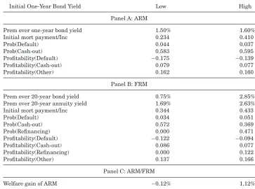
Turning to FRMs, in TableIIIwe see that, when initial interest rates are low, default rates for FRMs are lower than for ARMs. However, the reverse is true when initial interest rates are high. The reason is simple. When initial interest rates are high, mortgage providers must charge borrowers for the option to refinance the loan. This increases the premium and the average payments of FRMs, which makes them particularly expensive in an environment of declin-ing house prices and low interest rates. Negative home equity prevents borrow-ers from refinancing the loan, while low interest rates lead to a lower user cost of housing and lower rental payments compared to mortgage payments. On the other hand, for ARMs default tends to occur when nominal interest rates are high, since high interest rates lead to large mortgage payments.