Mastering Machine Learning
with R
Master machine learning techniques with R to deliver
insights for complex projects
Cory Lesmeister
Mastering Machine Learning with R
Copyright © 2015 Packt Publishing
All rights reserved. No part of this book may be reproduced, stored in a retrieval system, or transmitted in any form or by any means, without the prior written permission of the publisher, except in the case of brief quotations embedded in critical articles or reviews.
Every effort has been made in the preparation of this book to ensure the accuracy of the information presented. However, the information contained in this book is sold without warranty, either express or implied. Neither the author nor Packt Publishing, and its dealers and distributors will be held liable for any damages caused or alleged to be caused directly or indirectly by this book.
Packt Publishing has endeavored to provide trademark information about all of the companies and products mentioned in this book by the appropriate use of capitals. However, Packt Publishing cannot guarantee the accuracy of this information.
First published: October 2015
Production reference: 1231015
Published by Packt Publishing Ltd. Livery Place
35 Livery Street
Birmingham B3 2PB, UK. ISBN 978-1-78398-452-7
About the Author
About the Reviewers
Vikram Dhillon is a software developer, bioinformatics researcher, and software
coach at the Blackstone LaunchPad in the University of Central Florida. He has been working on his own start-up involving healthcare data security. He lives in Orlando and regularly attends developer meetups and hackathons. He enjoys spending his spare time reading about new technologies such as the blockchain and developing tutorials for machine learning in game design. He has been involved in open source projects for over 5 years and writes about technology and start-ups at opsbug.com.Miro Kopecky
is a passionate JVM enthusiast from the first moment he joined Sun Microsystems in 2002. Miro truly believes in a distributed system design, concurrency, and parallel computing, which means pushing the system's performance to its limits without losing reliability and stability. He has been working on research of new data mining techniques in neurological signal analysis during his PhD studies. Miro's hobbies include autonomic system development and robotics.Pavan Narayanan is an applied mathematician and is experienced in
mathematical programming, analytics, and web development. He has published and presented papers in algorithmic research to the Transportation Research Board, Washington DC and SUNY Research Conference, Albany, NY. An avid blogger at https://datasciencehacks.wordpress.com, his interests are exploring problem solving techniques—from industrial mathematics to machine learning. Pavan can be contacted at [email protected].
He has worked on books such as Apache mahout essentials, Learning apache mahout, and Real-time applications development with Storm and Petrel.
I would like to thank my family and God Almighty for giving me strength and endurance and the folks at Packt Publishing for the opportunity to work on this book.
Doug Ortiz is an independent consultant who has been architecting, developing,
and integrating enterprise solutions throughout his whole career. Organizations that leverage his skillset have been able to rediscover and reuse their underutilized data via existing and emerging technologies such as Microsoft BI Stack, Hadoop, NOSQL Databases, SharePoint, Hadoop, and related toolsets and technologies.Doug has experience in integrating multiple platforms and products. He has helped organizations gain a deeper understanding and value of their current investments in data and existing resources turning them into useful sources of information. He has improved, salvaged, and architected projects by utilizing unique and innovative techniques.
www.PacktPub.com
Support files, eBooks, discount offers, and more
For support files and downloads related to your book, please visit www.PacktPub.com.
Did you know that Packt offers eBook versions of every book published, with PDF and ePub files available? You can upgrade to the eBook version at www.PacktPub. com and as a print book customer, you are entitled to a discount on the eBook copy. Get in touch with us at [email protected] for more details.
At www.PacktPub.com, you can also read a collection of free technical articles, sign up for a range of free newsletters and receive exclusive discounts and offers on Packt books and eBooks.
TM
https://www2.packtpub.com/books/subscription/packtlib
Do you need instant solutions to your IT questions? PacktLib is Packt's online digital book library. Here, you can search, access, and read Packt's entire library of books.
Why subscribe?
• Fully searchable across every book published by Packt • Copy and paste, print, and bookmark content
• On demand and accessible via a web browser
Free access for Packt account holders
Table of Contents
Preface vii
Chapter 1: A Process for Success
1
The process 2
Business understanding 3
Identify the business objective 4
Assess the situation 5
Determine the analytical goals 5 Produce a project plan 5
Data understanding 6
Data preparation 6
Modeling 7 Evaluation 8 Deployment 8
Algorithm flowchart 9
Summary 14
Chapter 2:
Linear Regression – The Blocking and Tackling of
Machine Learning
15
Univariate linear regression 16
Business understanding 18
Multivariate linear regression 25
Business understanding 25 Data understanding and preparation 25 Modeling and evaluation 28
Other linear model considerations 40
Qualitative feature 41
Interaction term 43
Table of Contents
Chapter 3:
Logistic Regression and Discriminant Analysis
45
Classification methods and linear regression 46
Logistic regression 46
Business understanding 47 Data understanding and preparation 48 Modeling and evaluation 54
The logistic regression model 54
Logistic regression with cross-validation 58
Discriminant analysis overview 62 Discriminant analysis application 64
Model selection 69
Summary 74
Chapter 4: Advanced Feature Selection in Linear Models
75
Regularization in a nutshell 76
Ridge regression 77
LASSO 77
Elastic net 78
Business case 78
Business understanding 78 Data understanding and preparation 79
Modeling and evaluation 85
Chapter 5:
More Classification Techniques – K-Nearest
Neighbors and Support Vector Machines
105
K-Nearest Neighbors 106 Support Vector Machines 107
Business case 111
Business understanding 111 Data understanding and preparation 112 Modeling and evaluation 118
KNN modeling 118
SVM modeling 124
Table of Contents
Chapter 6:
Classification and Regression Trees
135
Introduction 135
An overview of the techniques 136
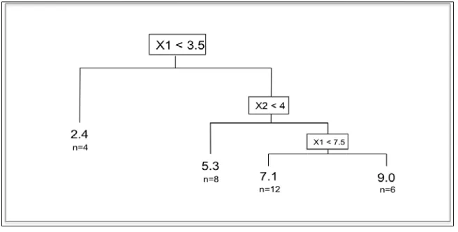
Regression trees 136
Chapter 7:
Neural Networks
165
Neural network 166
Deep learning, a not-so-deep overview 170 Business understanding 172 Data understanding and preparation 173 Modeling and evaluation 179
An example of deep learning 186
H2O background 187
Data preparation and uploading it to H2O 187 Create train and test datasets 191 Modeling 191
Summary 194
Chapter 8:
Cluster Analysis
195
Hierarchical clustering 196
Distance calculations 197
K-means clustering 198 Gower and partitioning around medoids 199
Gower 199 PAM 200 Business understanding 200
Data understanding and preparation 201
Modeling and evaluation 203
Table of Contents
Clustering with mixed data 217
Summary 220
Chapter 9:
Principal Components Analysis
221
An overview of the principal components 222
Rotation 225 Business understanding 226 Data understanding and preparation 227
Modeling and evaluation 233
Component extraction 233 Orthogonal rotation and interpretation 236 Creating factor scores from the components 237
Regression analysis 239
Summary 244
Chapter 10:
Market Basket Analysis and Recommendation
Engines 245
An overview of a market basket analysis 246
Business understanding 247
Data understanding and preparation 248
Modeling and evaluation 250
An overview of a recommendation engine 255
User-based collaborative filtering 256 Item-based collaborative filtering 257
Singular value decomposition and principal components analysis 257
Business understanding and recommendations 262 Data understanding, preparation, and recommendations 262 Modeling, evaluation, and recommendations 265
Summary 276
Chapter 11: Time Series and Causality
277
Univariate time series analysis 278
Bivariate regression 283
Granger causality 284
Business understanding 286 Data understanding and preparation 289
Modeling and evaluation 293
Univariate time series forecasting 294 Time series regression 302
Examining the causality 310
Table of Contents
Chapter 12:
Text Mining
319
Text mining framework and methods 320
Topic models 322
Other quantitative analyses 323 Business understanding 325 Data understanding and preparation 325
Modeling and evaluation 330
Word frequency and topic models 330 Additional quantitative analysis 337
Summary 344
Appendix:
R Fundamentals
345
Introduction 345
Getting R up and running 345
Using R 354
Data frames and matrices 358
Summary stats 360
Installing and loading the R packages 364
Summary 365
Preface
"He who defends everything, defends nothing."
— Frederick the Great
Machine learning is a very broad topic. The following quote sums it up nicely: The first problem facing you is the bewildering variety of learning algorithms available. Which one to use? There are literally thousands available, and hundreds more are published each year. (Domingo, P., 2012.) It would therefore be irresponsible to try and cover everything in the chapters that follow because, to paraphrase Frederick the Great, we would achieve nothing.
With this constraint in mind, I hope to provide a solid foundation of algorithms and business considerations that will allow the reader to walk away and, first of all, take on any machine learning tasks with complete confidence, and secondly, be able to help themselves in figuring out other algorithms and topics. Essentially, if this book significantly helps you to help yourself, then I would consider this a victory. Don't think of this book as a destination but rather, as a path to self-discovery.
Preface
Another thing that lit a fire under me to write this book was an incident that
happened in the hallways of a former employer a couple of years ago. My team had an IT contractor to support the management of our databases. As we were walking and chatting about big data and the like, he mentioned that he had bought a book about machine learning with R and another about machine learning with Python. He stated that he could do all the programming, but all of the statistics made absolutely no sense to him. I have always kept this conversation at the back of my mind
throughout the writing process. It has been a very challenging task to balance the technical and theoretical with the practical. One could, and probably someone has, turned the theory of each chapter to its own book. I used a heuristic of sorts to aid me in deciding whether a formula or technical aspect was in the scope, which was would this help me or the readers in the discussions with team members and business leaders? If I felt it might help, I would strive to provide the necessary details.
I also made a conscious effort to keep the datasets used in the practical exercises large enough to be interesting but small enough to allow you to gain insight without becoming overwhelmed. This book is not about big data, but make no mistake about it, the methods and concepts that we will discuss can be scaled to big data.
In short, this book will appeal to a broad group of individuals, from IT experts seeking to understand and interpret machine learning algorithms to statistical gurus desiring to incorporate the power of R into their analysis. However, even those that are well-versed in both IT and statistics—experts if you will—should be able to pick up quite a few tips and tricks to assist them in their efforts.
Machine learning defined
Machine learning is everywhere! It is used in web search, spam filters,
recommendation engines, medical diagnostics, ad placement, fraud detection, credit scoring, and I fear in these autonomous cars that I hear so much about. The roads are dangerous enough now; the idea of cars with artificial intelligence, requiring CTRL + ALT + DEL every 100 miles, aimlessly roaming the highways and byways is just too terrifying to contemplate. But, I digress.
It is always important to properly define what one is talking about and machine learning is no different. The website, machinelearningmastery.com, has a full page dedicated to this question, which provides some excellent background material. It also offers a succinct one-liner that is worth adopting as an operational definition:
Preface
With this definition in mind, we will require a few things in order to perform machine learning. The first is that we have the data. The second is that a pattern actually exists, which is to say that with known input values from our training data, we can make a prediction or decision based on data that we did not use to train the model. This is the generalization in machine learning. Third, we need some sort of performance measure to see how well we are learning/generalizing, for example, the mean squared error, accuracy, and others. We will look at a number of performance measures throughout the book.
One of the things that I find interesting in the world of machine learning are the changes in the language to describe the data and process. As such, I can't help but include this snippet from the philosopher, George Carlin:
"I wasn't notified of this. No one asked me if I agreed with it. It just happened. Toilet paper became bathroom tissue. Sneakers became running shoes. False teeth became dental appliances. Medicine became medication. Information became directory assistance. The dump became the landfill. Car crashes became automobile accidents. Partly cloudy became partly sunny. Motels became motor lodges. House trailers became mobile homes. Used cars became previously owned transportation. Room service became guest-room dining, and constipation became occasional irregularity.
— Philosopher and Comedian, George Carlin
I cut my teeth on datasets that had dependent and independent variables. I would build a model with the goal of trying to find the best fit. Now, I have labeled the instances and input features that require engineering, which will become the feature space that I use to learn a model. When all was said and done, I used to look at my model parameters; now, I look at weights.
The bottom line is that I still use these terms interchangeably and probably always will. Machine learning purists may curse me, but I don't believe I have caused any harm to life or limb.
Machine learning caveats
Preface
Failure to engineer features
Just throwing data at the problem is not enough; no matter how much of it exists. This may seem obvious, but I have personally experienced, and I know of others who have run into this problem, where business leaders assumed that providing vast amounts of raw data combined with the supposed magic of machine learning would solve all the problems. This is one of the reasons the first chapter is focused on a process that properly frames the business problem and leader's expectations. Unless you have data from a designed experiment or it has been already
preprocessed, raw, observational data will probably never be in a form that you can begin modeling. In any project, very little time is actually spent on building models. The most time-consuming activities will be on the engineering features: gathering, integrating, cleaning, and understanding the data. In the practical exercises in this book, I would estimate that 90 percent of my time was spent on coding these activities versus modeling. This, in an environment where most of the datasets are small and easily accessed. In my current role, 99 percent of the time in SAS is spent using PROC SQL and only 1 percent with things such as PROC GENMOD, PROC LOGISTIC, or Enterprise Miner.
When it comes to feature engineering, I fall in the camp of those that say there is no substitute for domain expertise. There seems to be another camp that believes machine learning algorithms can indeed automate most of the feature selection/engineering tasks and several start-ups are out to prove this very thing. (I have had discussions with a couple of individuals that purport their methodology does exactly that but they were closely guarded secrets.) Let's say that you have several hundred candidate features (independent variables). A way to perform automated feature selection is to compute the univariate information value. However, a feature that appears totally irrelevant in isolation can become important in combination with another feature. So, to get around this, you create numerous combinations of the features. This has potential problems of its own as you may have a dramatically increased computational time and cost and/or overfit your model. Speaking of overfitting, let's pursue it as the next caveat.
Overfitting and underfitting
Preface
Let's nail down the definitions. A bias error is the difference between the value or class that we predict and the actual value or class in our training data. A variance error is the amount by which the predicted value or class in our training set differs from the predicted value or class versus the other datasets. Of course, our goal is to minimize the total error (bias + variance), but how does that relate to model complexity?
For the sake of argument, let's say that we are trying to predict a value and we build a simple linear model with our train data. As this is a simple model, we could expect a high bias, while on the other hand, it would have a low variance between the train and test data. Now, let's try including polynomial terms in the linear model or build decision trees. The models are more complex and should reduce the bias. However, as the bias decreases, the variance, at some point, begins to expand and generalizability is diminished. You can see this phenomena in the following illustration. Any machine learning effort should strive to achieve the optimal trade-off between the bias and variance, which is easier said than done.
Preface
Causality
It seems a safe assumption that the proverbial correlation does not equal
causation—a dead horse has been sufficiently beaten. Or has it? It is quite apparent that correlation-to-causation leaps of faith are still an issue in the real world. As a result, we must remember and convey with conviction that these algorithms are based on observational and not experimental data. Regardless of what correlations we find via machine learning, nothing can trump a proper experimental design. As Professor Domingos states:
If we find that beer and diapers are often bought together at the supermarket, then perhaps putting beer next to the diaper section will increase sales. But short of actually doing the experiment it's difficult to tell."
— Domingos, P., 2012)
In Chapter 11, Time Series and Causality, we will touch on a technique borrowed from econometrics to explore causality in time series, tackling an emotionally and politically sensitive issue.
Enough of my waxing philosophically; let's get started with using R to master machine learning! If you are a complete novice to the R programming language, then I would recommend that you skip ahead and read the appendix on using R. Regardless of where you start reading, remember that this book is about the journey to master machine learning and not a destination in and of itself. As long as we are working in this field, there will always be something new and exciting to explore. As such, I look forward to receiving your comments, thoughts, suggestions, complaints, and grievances. As per the words of the Sioux warriors: Hoka-hey! (Loosely
translated it means forward together)
What this book covers
Chapter 1, A Process for Success - shows that machine learning is more than just writing code. In order for your efforts to achieve a lasting change in the industry, a proven process will be presented that will set you up for success.
Chapter 2, Linear Regression - The Blocking and Tackling of Machine Learning, provides you with a solid foundation before learning advanced methods such as Support Vector Machines and Gradient Boosting. No more solid foundation exists than the least squares linear regression.
Preface
Chapter 4, Advanced Feature Selection in Linear Models, shows regularization techniques to help improve the predictive ability and interpretability as feature selection is a critical and often extremely challenging component of machine learning.
Chapter 5, More Classification Techniques – K-Nearest Neighbors and Support Vector Machines, begins the exploration of the more advanced and nonlinear techniques. The real power of machine learning will be unveiled.
Chapter 6, Classification and Regression Trees, offers some of the most powerful
predictive abilities of all the machine learning techniques, especially for classification problems. Single decision trees will be discussed along with the more advanced random forests and boosted trees.
Chapter 7, Neural Networks, shows some of the most exciting machine learning methods currently used. Inspired by how the brain works, neural networks and their more recent and advanced offshoot, Deep Learning, will be put to the test. Chapter 8, Cluster Analysis, covers unsupervised learning. Instead of trying to make a prediction, the goal will focus on uncovering the latent structure of observations. Three clustering methods will be discussed: hierarchical, k-means, and partitioning around medoids.
Chapter 9, Principal Components Analysis, continues the examination of unsupervised learning with principal components analysis, which is used to uncover the latent structure of the features. Once this is done, the new features will be used in a supervised learning exercise.
Chapter 10, Market Basket Analysis and Recommendation Engines, presents the
techniques that are used to increase sales, detect fraud, and improve health. You will learn about market basket analysis of purchasing habits at a grocery store and then dig into building a recommendation engine on website reviews.
Chapter 11, Time Series and Causality, discusses univariate forecast models, bivariate regression, and Granger causality models, including an analysis of carbon emissions and climate change.
Chapter 12, Text Mining, demonstrates a framework for quantitative text mining and the building of topic models. Along with time series, the world of data contains vast volumes of data in a textual format. With so much data as text, it is critically important to understand how to manipulate, code, and analyze the data in order to provide meaningful insights.
Preface
What you need for this book
As R is a free and open source software, you will only need to download and install it from https://www.r-project.org/. Although it is not mandatory, it is highly recommended that you download IDE and RStudio from
https://www.rstudio.com/products/RStudio/.
Who this book is for
If you want to learn how to use R's machine learning capabilities in order to solve complex business problems, then this book is for you. An experience with R and a working knowledge of basic statistical or machine learning will prove helpful.
Conventions
In this book, you will find a number of text styles that distinguish between different kinds of information. Here are some examples of these styles and an explanation of their meaning.
Code words in text, database table names, folder names, filenames, file extensions, pathnames, dummy URLs, user input, and Twitter handles are shown as follows. Any command-line input or output is written as follows:
cor(x1, y1) #correlation of x1 and y1 [1] 0.8164205
> cor(x2, y1) #correlation of x2 and y2
[1] 0.8164205
New terms and important words are shown in bold. Words that you see on the screen, for example, in menus or dialog boxes, appear in the text like this: Clicking the Next button moves you to the next screen.
Warnings or important notes appear in a box like this.
Preface
Reader feedback
Feedback from our readers is always welcome. Let us know what you think about this book—what you liked or disliked. Reader feedback is important for us as it helps us develop titles that you will really get the most out of.
To send us general feedback, simply e-mail [email protected], and mention the book's title in the subject of your message.
If there is a topic that you have expertise in and you are interested in either writing or contributing to a book, see our author guide at www.packtpub.com/authors.
Customer support
Now that you are the proud owner of a Packt book, we have a number of things to help you to get the most from your purchase.
Downloading the example code
You can download the example code files from your account at http://www. packtpub.com for all the Packt Publishing books you have purchased. If you purchased this book elsewhere, you can visit http://www.packtpub.com/support
and register to have the files e-mailed directly to you.
Downloading the color images of this book
We also provide you with a PDF file that has color images of the screenshots/ diagrams used in this book. The color images will help you better understand the changes in the output. You can download this file from https://www.packtpub. com/sites/default/files/downloads/4527OS_ColouredImages.pdf.Errata
Although we have taken every care to ensure the accuracy of our content, mistakes do happen. If you find a mistake in one of our books—maybe a mistake in the text or the code—we would be grateful if you could report this to us. By doing so, you can save other readers from frustration and help us improve subsequent versions of this book. If you find any errata, please report them by visiting http://www.packtpub. com/submit-errata, selecting your book, clicking on the Errata Submission Form
Preface
To view the previously submitted errata, go to https://www.packtpub.com/books/ content/support and enter the name of the book in the search field. The required information will appear under the Errata section.
Piracy
Piracy of copyrighted material on the Internet is an ongoing problem across all media. At Packt, we take the protection of our copyright and licenses very seriously. If you come across any illegal copies of our works in any form on the Internet, please provide us with the location address or website name immediately so that we can pursue a remedy.
Please contact us at [email protected] with a link to the suspected pirated material.
We appreciate your help in protecting our authors and our ability to bring you valuable content.
eBooks, discount offers, and more
Did you know that Packt offers eBook versions of every book published, with PDF and ePub files available? You can upgrade to the eBook version at www.PacktPub. com and as a print book customer, you are entitled to a discount on the eBook copy. Get in touch with us at [email protected] for more details.
At www.PacktPub.com, you can also read a collection of free technical articles, sign up for a range of free newsletters, and receive exclusive discounts and offers on Packt books and eBooks.
Questions
A Process for Success
"If you don't know where you are going, any road will get you there."
— Robert Carrol
"If you can't describe what you are doing as a process, you don't know what you're doing."
— W. Edwards Deming At first glance, this chapter may seem to have nothing to do with machine learning, but it has everything to do with machine learning and specifically, its implementation and making the changes happen. The smartest people, best software, and best algorithm do not guarantee success, no matter how it is defined.
In most—if not all—projects, the key to successfully solving problems or improving decision-making is not the algorithm, but the soft, more qualitative skills of
A Process for Success
I will not hesitate to say that this all is easier said than done, and without question, I'm guilty of every sin by both commission and omission that will be discussed in this chapter. With skill and some luck, you can avoid the many physical and emotional scars I've picked up over the last 10 and a half years.
Finally, we will also have a look at a flow chart (a cheat sheet) that you can use to help you identify what methodology to apply to the problem at hand.
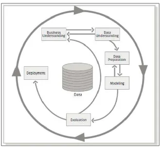
The process
Chapter 1
The process has the following six phases: • Business Understanding
• Data Understanding
• Data Preparation
• Modeling
• Evaluation
• Deployment
For an in-depth review of the entire process with all of its tasks and subtasks, you can examine the paper by SPSS, CRISP-DM 1.0, step-by-step data mining guide, available at https://the-modeling-agency.com/crisp-dm.pdf.
I will discuss each of the steps in the process, covering the important tasks. However, it will not be in the detailed level of the guide, but more high level. We will not skip any of the critical details but focus more on the techniques that one can apply to the tasks. Keep in mind that the process steps will be used in the later chapters as a framework in the actual application of the machine learning methods in general and the R code specifically.
Business understanding
One cannot underestimate how important this first step of the process is in achieving success. It is the foundational step and failure or success here will likely determine failure or success for the rest of the project. The purpose of this step is to identify the requirements of the business so that you can translate them into analytical objectives. It has the following four tasks:
1. Identify the business objective 2. Assess the situation
A Process for Success
Identify the business objective
The key to this task is to identify the goals of the organization and frame the problem. An effective question to ask is, what are we going to do different? This may seem like a benign question, but it can really challenge people to ponder what they need from an analytical perspective and it can get to the root of the decision that needs to be made. It can also prevent you from going out and doing a lot of unnecessary work on some fishing expedition. As such, the key for you is to identify the decision. A working definition of a decision can be put forward to the team
as the irrevocable choice to commit or not commit the resources. Additionally, remember that the choice to do nothing different is indeed a decision.
This does not mean that a project should not be launched if the choices are not absolutely clear. There will be times when the problem is not or cannot be well-defined; to paraphrase former Defense Secretary Donald Rumsfeld, there are known – unknowns. Indeed, there will probably be many times when the problem is ill-defined and the project's main goal is to further the understanding of the problem and generate hypotheses; again calling on Secretary Rumsfeld, unknown – unknowns, which means that you don't know what you don't know. However, in ill-defined problems, one should go forward with an understanding of what will happen next in terms of resource commitment based on the various outcomes of hypothesis exploration.
Another thing to consider in this task is to manage expectations. There is no such thing as a perfect data, no matter what its depth and breadth is. This is not the time to make guarantees but to communicate what is possible, given your expertise. I recommend a couple of outputs from this task. The first is a mission statement. This is not the touchy-feely mission statement of an organization, but it is your mission statement or, more importantly, the mission statement approved by the project sponsor. I stole this idea from my years of military experience and I could write volumes on why it is effective, but that is for another day. Let's just say that in the absence of clear direction or guidance, the mission statement or whatever you want to call it becomes the unifying statement and can help prevent scope creep. It consists of the following points:
• Who: This is yourself or the team or project name; everyone likes a cool project name, for example, Project Viper, Project Fusion, and so on
• What: This is the task that you will perform, for example, conduct machine learning
• When: This is the deadline
Chapter 1
The second task is to have as clear a definition of success as possible. Literally, ask what does success look like? Help the team/sponsor paint a picture of success that you can understand. Your job then is to translate this into modeling requirements.
Assess the situation
This task helps you in project planning by gathering information on the resources available, constraints, and assumptions, identifying the risks, and building
contingency plans. I would further add that this is also the time to identify the key stakeholders that will be impacted by the decisions to be made.
A couple of points here. When examining the resources that are available, do not neglect to scour the records of the past and current projects. Odds are someone in the organization has or is working on the same problem and it may be essential to synchronize your work with theirs. Don't forget to enumerate the risks considering time, people, and money. Do everything in your power to create a list of the stakeholders, both those that impact your project and those that could be impacted by your project. Identify who these people are and how they can influence/be impacted by the decision. Once this is done, work with the project sponsor to formulate a communication plan with these stakeholders.
Determine the analytical goals
Here, you are looking to translate the business goal into technical requirements. This includes turning the success criterion from the task of creating a business objective to technical success. This might be things such as RMSE or a level of predictive accuracy.
Produce a project plan
A Process for Success
Data understanding
After enduring the all-important pain of the first step, you can now get your hands on the data. The tasks in this process consist of the following:
1. Collect the data 2. Describe the data 3. Explore the data 4. Verify the data quality
This step is the classic case of ETL is Extract, Transform, Load. There are some considerations here. You need to make an initial determination that the data
available is adequate to meet your analytical needs. As you explore the data, visually and otherwise, determine if the variables are sparse and identify the extent to which the data may be missing. This may drive the learning method that you use and/or whether the imputation of the missing data is necessary and feasible.
Verifying the data quality is critical. Take the time to understand who collects the data, how it is collected, and even why it is collected. It is likely that you may stumble upon an incomplete data collection, cases where unintended IT issues led to errors in the data, or there were planned changes in the business rules. This is critical in the time series where often business rules change over time on how the data is classified. Finally, it is a good idea to begin documenting any code at this step. As a part of the documentation process, if a data dictionary is not available, save yourself the heartache later on and make one.
Data preparation
Almost there! This step has the following five tasks: 1. Select the data
Chapter 1
These tasks are relatively self-explanatory. The goal is to get the data ready to input in the algorithms. This includes merging, feature engineering, and transformations. If imputation is needed, then it happens here as well. Additionally, with R, pay attention to how the outcome needs to be labeled. If your outcome/response variable is Yes/No, it may not work in some packages and will require a transformed or no variable with 1/0. At this point, you should also break your data into the various test sets if applicable: train, test, or validate. This step can be an unforgivable burden, but most experienced people will tell you that it is where you can separate yourself from your peers. With this, let's move on to the money step.
Modeling
This is where all the work that you've done up to this point can lead to fist-pumping exuberance or fist-pounding exasperation. But hey, if it was that easy, everyone would be doing it. The tasks are as follows:
1. Select a modeling technique 2. Generate a test design 3. Build a model
4. Assess a model
Oddly, this process step includes the considerations that you have already thought of and prepared for. In the first step, one will need at least a modicum of an idea about how they will be modeling. Remember, that this is a flexible, iterative process and not some strict linear flowchart such as an aircrew checklist.
The cheat sheet included in this chapter should help guide you in the right direction for the modeling techniques. A test design refers to the creation of your test and train datasets and/or the use of cross-validation and this should have been thought of and accounted for in the data preparation.
A Process for Success
Evaluation
With the evaluation process, the main goal is to confirm that the work that has been done and the model selected at this point meets the business objective. Ask yourself and others, have we achieved the definition of success? Let the Netflix prize serve as a cautionary tale here. I'm sure you are aware that Netflix awarded a $1 million prize to the team that could produce the best recommendation algorithm as defined by the lowest RMSE. However, Netflix did not implement it because the incremental accuracy gained was not worth the engineering effort! Always apply Occam's razor. At any rate, here are the tasks:
1. Evaluate the results 2. Review the process 3. Determine the next steps
In reviewing the process, it may be necessary—as you no doubt determined earlier in the process—to take the results through governance and communicate with the other stakeholders in order to gain their buy-in. As for the next steps, if you want to be a change agent, make sure that you answer the what, so what, and now what in the stakeholders' minds. If you can tie their now what into the decision that you made earlier, you are money.
Deployment
If everything is done according to the plan up to this point, it might just come down to flipping a switch and your model goes live. Assuming that this is not the case, here are the tasks of this step:
1. Deploying the plan
2. Monitoring and maintenance of the plan 3. Producing the final report
4. Reviewing the project
Chapter 1
Now for the all-important process review. You may have your own proprietary way of conducting it, but here is what it should cover, whether you conduct it in a formal or informal way:
• What was the plan? • What actually happened?
• Why did it happen or did not happen? • What should be sustained in future projects? • What should be improved upon in future projects?
• Create an action plan to ensure sustainment and improvement happens That concludes the review of the CRISP-DM process, which provides a
comprehensive and flexible framework to guarantee the success of your project and make you an agent of change.
Algorithm flowchart
A Process for Success
The following figure starts the flow of selecting the potential modeling techniques. As you answer the question(s), it will take you to one of the four additional charts:
Chapter 1
If the data is a text or in the time series format, then you will follow the flow in the following figure:
A Process for Success
In this branch of the algorithm, you do not have a text or the time series data. Additionally, you are not trying to predict what category the observations belong to.
Chapter 1
To get to this section, you would have data that is not text or time series. You want to categorize the data, but it does not have an outcome label, which brings us to clustering methods, as follows:
Figure 4
A Process for Success
Summary
This chapter was about how to set yourself and your team up for success in any project that you tackle. The CRISP-DM process is put forward as a flexible and comprehensive framework in order to facilitate the softer skills of communication and influence. Each process step and the tasks in each step were enumerated. More than that, the commentary provides some techniques and considerations to help in the process execution. By taking heed of the process, you can indeed become an agent of positive change to any organization.
Linear Regression – The
Blocking and Tackling of
Machine Learning
"Some people try to find things in this game that don't exist, but football is only two things – blocking and tackling."
— Vince Lombardi, Hall of Fame Football Coach
Linear Regression – The Blocking and Tackling of Machine Learning
Univariate linear regression
We begin by looking at a simple way to predict a quantitative response, Y, with one predictor variable, x, assuming that Y has a linear relationship with x. The model for this can be written as, Y = B0 + B1x + e. We can state it as the expected value of Y being a function of the parameters B0 (the intercept) plus B1 (the slope) times x, plus an error term. The least squares approach chooses the model parameters that minimize the Residual Sum of Squares (RSS) of the predicted y values versus the actual Y values. For a simple example, let's say we have the actual values of Y1 and Y2 equal to 10 and 20 respectively, along with the predictions of y1 and y2 as 12 and 18. To calculate RSS, we add the squared differences RSS = (Y1 – y1)2 + (Y2 – y2)2,
which, with simple substitution, yields (10 – 12)2 + (20 – 18)2 = 8.
I once remarked to a peer during our Lean Six Sigma Black Belt training that it's all about the sum of squares; understand the sum of squares and the rest will flow naturally. Perhaps that is true, at least to some extent.
Before we begin with an application, I want to point out that if you read the
headlines of various research breakthroughs, do so with a jaded eye and a skeptical mind as the conclusion put forth by the media may not be valid. As we shall see, R, and any other software for that matter, will give us a solution regardless of the inputs. However, just because the math makes sense and a high correlation or R-squared statistic is reported, doesn't mean that the conclusion is valid.
To drive this point home, a look at the famous Anscombe dataset available in R is in order. The statistician Francis Anscombe produced this set to highlight the importance of data visualization and outliers when analyzing data. It consists of four pairs of X and Y variables that have the same statistical properties, but when plotted, show something very different. I have used the data to train colleagues and to educate business partners on the hazards of fixating on statistics without exploring the data and checking assumptions. I think this is a good place to start with the following R code should you have a similar need. It is a brief tangent before moving on to serious modeling.
> #call up and explore the data
> data(anscombe)
> attach(anscombe)
> anscombe
Chapter 2
As we shall see, each of the pairs has the same correlation coefficient of 0.816. The first two are as follows:
> cor(x1, y1) #correlation of x1 and y1 [1] 0.8164205
> cor(x2, y1) #correlation of x2 and y2
[1] 0.8164205
The real insight here, as Anscombe intended, is when we plot all the four pairs together, as follows:
> par(mfrow=c(2,2)) #create a 2x2 grid for plotting
> plot(x1, y1, main="Plot 1")
> plot(x2, y2, main="Plot 2")
> plot(x3, y3, main="Plot 3")
> plot(x4, y4, main="Plot 4")
Downloading the example code
You can download the example code files for all
Packt books you have purchased from your account at http://www.packtpub.com. If you purchased this book elsewhere, you can visit http://www. packtpub.com/support and register to have the
Linear Regression – The Blocking and Tackling of Machine Learning
The output of the preceding code is as follows:
As we can see, Plot 1 appears to have a true linear relationship, Plot 2 is curvilinear,
Plot 3 has a dangerous outlier, and Plot 4 is driven by the one outlier. There you have it, a cautionary tale of sorts.
Business understanding
The data collected measures two variables. The goal is to model the water yield (in inches) of the Snake River Watershed in Wyoming as a function of the water content of the year's snowfall. This forecast will be useful in managing the water flow and reservoir levels as the Snake River provides the much needed irrigation water for the farms and ranches of several western states. The dataset snake is available in the alr3 package (note that alr stands for applied linear regression):
> install.packages("alr3") > library(alr3)
Chapter 2
1 23.1 10.5 2 32.8 16.7 3 31.8 18.2 4 32.0 17.0 5 30.4 16.3 6 24.0 10.5
Now that we have 17 observations, data exploration can begin. But first, let's change X and Y into meaningful variable names, as follows:
> names(snake) = c("content", "yield")
> attach(snake) #reattach data with new names > head(snake)
content yield 1 23.1 10.5 2 32.8 16.7 3 31.8 18.2 4 32.0 17.0 5 30.4 16.3 6 24.0 10.5
> plot(content, yield, xlab="water content of snow", ylab="water yield")
Linear Regression – The Blocking and Tackling of Machine Learning
This is an interesting plot as the data is linear, and has a slight curvilinear shape driven by two potential outliers at both ends of the extreme. As a result, a
transformation of the data or deletion of an outlying observation may be warranted. To perform a linear regression in R, one uses the lm() function to create a model in the standard form of fit = lm(Y~X). You can then test your assumptions using various functions on your fitted model by using the following code:
> yield.fit = lm(yield~content) -2.1793 -1.5149 -0.3624 1.6276 3.1973
Coefficients:
Residual standard error: 1.743 on 15 degrees of freedom Multiple R-squared: 0.8709, Adjusted R-squared: 0.8623 F-statistic: 101.2 on 1 and 15 DF, p-value: 4.632e-08
Chapter 2
Since the p-value is highly significant, we can reject the null and move on to the t-test for content, which tests the null hypothesis that it is 0. Again, we can reject the null. Additionally, we can see Multiple R-squared and Adjusted R-squared values. The Adjusted R-squared will be covered under the multivariate regression topic, so let's zero in on Multiple R-squared; here we see that it is 0.8709. In theory, it can range from 0 to 1 and is a measure of the strength of the association between X and Y. The interpretation in this case is that 87 percent of the variation in the water yield can be explained by the water content of snow. On a side note, R-squared is nothing more than the correlation coefficient of [X, Y] squared.
We can recall our scatterplot, and now add the best fit line produced by our model using the following code:
> plot(content, yield)
> abline(yield.fit, lwd=3, col="red")
Linear Regression – The Blocking and Tackling of Machine Learning
A linear regression model is only as good as the validity of its assumptions, which can be summarized as follows:
• Linearity: This is a linear relationship between the predictor and the
response variables. If this relationship is not clearly present, transformations (log, polynomial, exponent and so on) of the X or Y may solve the problem. • Non-correlation of errors: A common problem in the time series and panel
data where en = betan-1; if the errors are correlated, you run the risk of creating a poorly specified model.
• Homoscedasticity: Normally the distributed and constant variance of errors, which means that the variance of the errors is constant across the different values of inputs. Violations of this assumption can create biased coefficient estimates, leading to statistical tests for significance that can be either too high or too low. This, in turn, leads to the wrong conclusion. This violation is referred to as heteroscedasticity.
• No collinearity: No linear relationship between two predictor variables, which is to say that there should be no correlation between the features. This, again, can lead to biased estimates.
• Presence of outliers: Outliers can severely skew the estimation and, ideally, must be removed prior to fitting a model using linear regression; this again can lead to a biased estimate.
As we are building a univariate model not dependent on time, we will concern ourselves only with linearity and heteroscedasticity. The other assumptions will become important in the next section. The best way to initially check the assumptions is by producing plots. The plot() function, when combined with a linear model fit, will automatically produce four plots allowing you to examine the assumptions. R produces the plots one at a time and you advance through them by hitting the Enter key. It is best to examine all four simultaneously and we do it in the following manner: > par(mfrow=c(2,2))
Chapter 2
The output of the preceding code is as follows:
The two plots on the left allow us to examine the homoscedasticity of errors and nonlinearity. What we are looking for is some type of pattern or, more importantly, that no pattern exists. Given the sample size of only 17 observations, nothing obvious can be seen. Common heteroscedastic errors will appear to be u-shaped, inverted u-shaped, or will cluster close together on the left side of the plot and become wider as the fitted values increase (a funnel shape). It is safe to conclude that no violation of homoscedasticity is apparent in our model.
Linear Regression – The Blocking and Tackling of Machine Learning
What exactly is further inspection? This is where art meets science. The easy way out would be to simply delete the observation, in this case number 9, and redo the model. However, a better option may be to transform the predictor and/or the response variables. If we just delete observation 9, then maybe observations 10 and
13 would fall outside the band of greater than 1. I believe that this is where domain expertise can be critical. More times than I can count, I have found that exploring and understanding the outliers can yield valuable insights. When we first examined the previous scatterplot I pointed out the potential outliers and these happen to be observations number 9 and number 13. As an analyst, it would be critical to discuss with the appropriate subject matter experts to understand why this would be the case. Is it a measurement error? Is there a logical explanation for these observations? I certainly don't know, but this is an opportunity to increase the value that you bring to an organization.
Having said that, we can drill down on the current model by examining, in more detail, the Normal Q-Q plot. R does not provide confidence intervals to the default
Q-Q plot, and given our concerns in looking at the base plot, we should check the confidence intervals. The qqPlot() function of the car package automatically provides these confidence intervals. Since the car package is loaded along with the alr3 package, I can produce the plot with one line of code as follows:
> qqPlot(yield.fit)
Chapter 2
According to the plot, the residuals are normally distributed. I think this can give us some confidence to select the model with all the observations. Clear rationale and judgment would be needed to attempt other models. If we could clearly reject the assumption of normally distributed errors, then we would probably have to examine the variable transformations and/or observation deletion.
Multivariate linear regression
You may be asking yourself the question if in the real world you would ever have just one predictor variable; that is, indeed, fair. Most likely, several, if not many, predictor variables or features, as they are affectionately termed in machine learning, will have to be included in your model. And with that, let's move on to multivariate linear regression and a new business case.
Business understanding
In keeping with the water conservation/prediction theme, let's look at another dataset in the alr3 package, appropriately named water. Lately, the severe drought in Southern California has caused much alarm. Even the Governor, Jerry Brown, has begun to take action with a call to citizens to reduce water usage by 20 percent. For this exercise, let's say we have been commissioned by the state of California to predict water availability. The data provided to us contains 43 years of snow precipitation, measured at six different sites in the Owens Valley. It also contains a response variable for water availability as the stream runoff volume near Bishop, California, which feeds into the Owens Valley aqueduct, and eventually, the Los Angeles Aqueduct. Accurate predictions of the stream runoff will allow engineers, planners, and policy makers to plan conservation measures more effectively. The model we are looking to create will consist of the form Y = B0 + B1x1 +...Bnxn + e, where the predictor variables (features) can be from 1 to n.
Data understanding and preparation
To begin, we will load the dataset named water and define the structure of the str() function as follows:
> data(water)
> str(water)
'data.frame': 43 obs. of 8 variables:
Linear Regression – The Blocking and Tackling of Machine Learning
$ APSLAKE: num 3.91 5.2 3.67 3.93 4.88 4.91 1.77 6.51 3.38 4.08 ... $ OPBPC : num 4.1 7.55 9.52 11.14 16.34 ...
$ OPRC : num 7.43 11.11 12.2 15.15 20.05 ... $ OPSLAKE: num 6.47 10.26 11.35 11.13 22.81 ...
$ BSAAM : int 54235 67567 66161 68094 107080 67594 65356 67909 92715 70024 ...
Here we have eight features and one response variable, BSAAM. The observations start in 1943 and run for 43 consecutive years. Since we are not concerned with what year the observations occurred, it makes sense to create a new data frame, excluding the year vector. This is quite easy to do. With one line of code, we can create the new data frame, and then verify that it worked with the head() function as follows: > socal.water = water[ ,-1] #new dataframe with the deletion of column 1
> head(socal.water)
APMAM APSAB APSLAKE OPBPC OPRC OPSLAKE BSAAM 1 9.13 3.58 3.91 4.10 7.43 6.47 54235
With all the features being quantitative, it makes sense to look at the correlation statistics and then produce a matrix of scatterplots. The correlation coefficient or
Pearson's r, is a measure of both the strength and direction of the linear relationship between two variables. The statistic will be a number between -1 and 1 where -1 is the total negative correlation and +1 is the total positive correlation. The calculation of the coefficient is the covariance of the two variables, divided by the product of their standard deviations. As previously discussed, if you square the correlation coefficient, you will end up with R-squared.
Chapter 2
> water.cor = cor(socal.water)
> water.cor
APMAM APSAB APSLAKE OPBPC APMAM 1.0000000 0.82768637 0.81607595 0.12238567
APSAB 0.8276864 1.00000000 0.90030474 0.03954211 APSLAKE 0.8160760 0.90030474 1.00000000 0.09344773 OPBPC 0.1223857 0.03954211 0.09344773 1.00000000 OPRC 0.1544155 0.10563959 0.10638359 0.86470733 OPSLAKE 0.1075421 0.02961175 0.10058669 0.94334741 BSAAM 0.2385695 0.18329499 0.24934094 0.88574778 OPRC OPSLAKE BSAAM
APMAM 0.1544155 0.10754212 0.2385695 APSAB 0.1056396 0.02961175 0.1832950 APSLAKE 0.1063836 0.10058669 0.2493409 OPBPC 0.8647073 0.94334741 0.8857478 OPRC 1.0000000 0.91914467 0.9196270 OPSLAKE 0.9191447 1.00000000 0.9384360 BSAAM 0.9196270 0.93843604 1.0000000
So, what does this tell us? First of all, the response variable is highly and positively correlated with the OP features with OPBPC as 0.8857, OPRC as 0.9196, and
OPSLAKE as 0.9384. Also note that the AP features are highly correlated with each other and the OP features as well. The implication is that we may run into the issue of multicollinearity. The correlation plot matrix provides a nice visual of the correlations as follows:
Linear Regression – The Blocking and Tackling of Machine Learning
The output of the preceding code snippet is as follows:
Modeling and evaluation
One of the key elements that we will cover here is the very important task of feature selection. In this chapter, we will discuss the best subsets regression methods stepwise, using the leaps package. The later chapters will cover more advanced techniques.
Forward stepwise selection starts with a model that has zero features; it then adds the features one at a time until all the features are added. A selected feature is added in the process that creates a model with the lowest RSS. So in theory, the first feature selected should be the one that explains the response variable better than any of the others, and so on.
It is important to note that adding a feature will always decrease RSS and increase R-squared, but will not necessarily improve the model fit and interpretability.
Chapter 2
It is important to add here that stepwise techniques can suffer from serious issues. You can perform a forward stepwise on a dataset, then a backward stepwise, and end up with two completely conflicting models. The bottom line is that stepwise can produce biased regression coefficients; in other words, they are too large and the confidence intervals are too narrow (Tibrishani, 1996).
Best subsets regression can be a satisfactory alternative to the stepwise methods for feature selection. In best subsets regression, the algorithm fits a model for all the possible feature combinations; so if you have 3 features, 23 models will be created. As with stepwise regression, the analyst will need to apply judgment or statistical analysis to select the optimal model. Model selection will be the key topic in the discussion that follows. As you might have guessed, if your dataset has many features, this can be quite a task, and the method does not perform well when you have more features than observations (p is greater than n).
Certainly, these limitations for best subsets do not apply to our task at hand. Given its limitations, we will forgo stepwise, but please feel free to give it a try. We will begin by loading the leaps package. In order that we may see how feature selection works, we will first build and examine a model with all the features, then drill down with best subsets to select the best fit.
To build a linear model with all the features, we can again use the lm() function. It will follow the form: fit = lm(y ~ x1 + x2 + x3...xn). A neat shortcut, if you want to include all the features, is to use a period after the tilde symbol instead of having to type them all in. For starters, let's load the leaps package and build a model with all the features for examination as follows:
> library(leaps)
> fit=lm(BSAAM~., data=socal.water)
> summary(fit)
Call:
lm(formula = BSAAM ~ ., data = socal.water)
Residuals:
Linear Regression – The Blocking and Tackling of Machine Learning
Estimate Std. Error t value Pr(>|t|) (Intercept) 15944.67 4099.80 3.889 0.000416 *** APMAM -12.77 708.89 -0.018 0.985725
Residual standard error: 7557 on 36 degrees of freedom Multiple R-squared: 0.9248, Adjusted R-squared: 0.9123 F-statistic: 73.82 on 6 and 36 DF, p-value: < 2.2e-16
Just like with univariate regression, we examine the p-value on the F-statistic
to see if at least one of the coefficients is not zero and, indeed, the p-value is highly significant. We should also have significant p-values for the OPRC and OPSLAKE parameters. Interestingly, OPBPC is not significant despite being highly correlated with the response variable. In short, when we control for the other OP features, OPBPC no longer explains any meaningful variation of the predictor, which is to say that the feature OPBPC adds nothing from a statistical standpoint with OPRC and OPSLAKE in the model.
With the first model built, let's move on to best subsets. We create the sub.fit object using the regsubsets() function of the leaps package as follows:
> sub.fit = regsubsets(BSAAM~., data=socal.water)
Then we create the best.summary object to examine the models further. As with all R objects, you can use the names() function to list what outputs are available, as follows:
> best.summary = summary(sub.fit)
> names(best.summary)
[1] "which" "rsq" "rss" "adjr2" "cp" "bic" "outmat" "obj"
Chapter 2
The code tells us that the model with six features has the smallest RSS, which it should have, as that is the maximum number of inputs and more inputs mean a lower RSS. An important point here is that adding features will always decrease RSS! Furthermore, it will always increase R-squared. We could add a completely irrelevant feature like the number of wins for the Los Angeles Lakers and RSS would decrease and R-squared would increase. The amount would likely be miniscule, but present nonetheless. As such, we need an effective method to properly select the relevant features.
For feature selection, there are four statistical methods that we will talk about in this chapter: Aikake's Information Criterion (AIC), Mallow's Cp (Cp), Bayesian Information Criterion (BIC), and the adjusted R-squared. With the first three, the
goal is to minimize the value of the statistic; with adjusted R-squared, the goal is to maximize the statistics value. The purpose of these statistics is to create as parsimonious a model as possible, in other words, penalize model complexity. The formulation of these four statistics is as follows:
• log RSSp 2
testing and MSEf is the mean of the squared error of the model, with all features included and n is the sample size
• log RSSp log( )
model we are testing and n is the sample size
In a linear model, AIC and Cp are proportional to each other, so we will only concern ourselves with Cp, which follows the output available in the leaps package. BIC tends to select the models with fewer variables than Cp, so we will compare both. To do so, we can create and analyze two plots side by side. Let's do this for Cp followed by BIC with the help of following code snippet:
> par(mfrow=c(1,2))
> plot(best.summary$cp, xlab="number of features", ylab="cp")
Linear Regression – The Blocking and Tackling of Machine Learning
The output of preceding code snippet is as follows:
In the plot on the left-hand side, the model with three features has the lowest cp. The plot on the right-hand side displays those features that provide the lowest Cp. The way to read this plot is to select the lowest Cp value at the top of the y axis, which is 1.2. Then, move to the right and look at the colored blocks corresponding to the x axis. Doing this, we see that APSLAKE, OPRC, and OPSLAKE are the features included in this specific model. By using the which.min() and which.max() functions, we can identify how cp compares to BIC and the adjusted R-squared. > which.min(best.summary$bic)
[1] 3
> which.max(best.summary$adjr2) [1] 3
In this example, BIC and adjusted R-squared match the Cp for the optimal model. Now, just like with univariate regression, we need to examine the model and test the assumptions. We'll do this by creating a linear model object and examining the plots in a similar fashion to what we did earlier, as follows:
> best.fit = lm(BSAAM~APSLAKE+OPRC+OPSLAKE, data=socal.water)
> summary(best.fit) Call:
Chapter 2
Min 1Q Median 3Q Max -12964 -5140 -1252 4446 18649
Coefficients:
Estimate Std. Error t value Pr(>|t|) (Intercept) 15424.6 3638.4 4.239 0.000133 *** APSLAKE 1712.5 500.5 3.421 0.001475 ** OPRC 1797.5 567.8 3.166 0.002998 ** OPSLAKE 2389.8 447.1 5.346 4.19e-06 ***
---Signif. codes: 0 '***' 0.001 '**' 0.01 '*' 0.05 '.' 0.1 ' ' 1
Residual standard error: 7284 on 39 degrees of freedom Multiple R-squared: 0.9244, Adjusted R-squared: 0.9185 F-statistic: 158.9 on 3 and 39 DF, p-value: < 2.2e-16
With the three-feature model, F-statistic and all the t-tests have significant p-values. Having passed the first test, we can produce our diagnostic plots:
> par(mfrow=c(2,2))
> plot(best.fit)

![Figure 2[ 11 ]](https://thumb-ap.123doks.com/thumbv2/123dok/3939686.1883106/36.612.126.488.147.542/figure.webp)
![Figure 3[ 12 ]](https://thumb-ap.123doks.com/thumbv2/123dok/3939686.1883106/37.612.126.490.150.539/figure.webp)
![Figure 5[ 13 ]](https://thumb-ap.123doks.com/thumbv2/123dok/3939686.1883106/38.612.214.400.164.365/figure.webp)