Effective Multi-Tenant Distributed Systems
Challenges and Solutions when Running Complex Environments
Effective Multi-Tenant Distributed Systems
by Chad Carson and Sean Suchter
Copyright © 2017 Pepperdata, Inc. All rights reserved. Printed in the United States of America.
Published by O’Reilly Media, Inc., 1005 Gravenstein Highway North, Sebastopol, CA 95472. O’Reilly books may be purchased for educational, business, or sales promotional use. Online editions are also available for most titles (http://safaribooksonline.com). For more information, contact our corporate/institutional sales department: 800-998-9938 or [email protected].
Editor: Nicole Taché and Debbie Hardin
Production Editor: Nicholas Adams
Copyeditor: Octal Publishing Inc.
Interior Designer: David Futato
Cover Designer: Randy Comer
Illustrator: Rebecca Demarest
October 2016: First Edition
Revision History for the First Edition
2016-10-10: First Release
The O’Reilly logo is a registered trademark of O’Reilly Media, Inc. Effective Multi-Tenant
Distributed Systems, the cover image, and related trade dress are trademarks of O’Reilly Media, Inc. While the publisher and the authors have used good faith efforts to ensure that the information and instructions contained in this work are accurate, the publisher and the authors disclaim all
responsibility for errors or omissions, including without limitation responsibility for damages
resulting from the use of or reliance on this work. Use of the information and instructions contained in this work is at your own risk. If any code samples or other technology this work contains or describes is subject to open source licenses or the intellectual property rights of others, it is your responsibility to ensure that your use thereof complies with such licenses and/or rights.
Chapter 1. Introduction to Multi-Tenant
Distributed Systems
The Benefits of Distributed Systems
The past few decades have seen an explosion of computing power. Search engines, social networks, cloud-based storage and computing, and similar services now make seemingly infinite amounts of information and computation available to users across the globe.
The tremendous scale of these services would not be possible without distributed systems. Distributed systems make it possible for many hundreds or thousands of relatively inexpensive
computers to communicate with one another and work together, creating the outward appearance of a single, high-powered computer. The primary benefit of a distributed system is clear: the ability to massively scale computing power relatively inexpensively, enabling organizations to scale up their businesses to a global level in a way that was not possible even a decade ago.
Performance Problems in Distributed Systems
As more and more nodes are added to the distributed system and interact with one another, and as more and more developers write and run applications on the system, complications arise. Operators of distributed systems must address an array of challenges that affect the performance of the system as a whole as well as individual applications’ performance.
These performance challenges are different from those faced when operating a data center of computers that are running more or less independently, such as a web server farm. In a true
distributed system, applications are split into smaller units of work, which are spread across many nodes and communicate with one another either directly or via shared input/output data.
Additional performance challenges arise with multi-tenant distributed systems, in which different users, groups, and possibly business units run different applications on the same cluster. (This is in contrast to a single, large distributed application, such as a search engine, which is quite complex and has intertask dependencies but is still just one overall application.) These challenges that come with multitenancy result from the diversity of applications running together on any node as well as the fact that the applications are written by many different developers instead of one engineering team focused on ensuring that everything in a single distributed application works well together.
Scheduling
must decide which jobs should be scheduled to run where and when, and the relative priority of those jobs. Even sophisticated distributed-system schedulers have limitations that can lead to
underutilization of cluster hardware, unpredictable job run times, or both. Examples include assuming the worst-case resource usage to avoid overcommitting, failing to plan for different resource types across different applications, and overlooking one or more dependencies, thus causing deadlock or starvation.
The scheduling challenges become more severe on multi-tenant clusters, which add fairness of
resource access among users as a scheduling goal, in addition to (and often in conflict with) the goals of high overall hardware utilization and predictable run times for high-priority applications. Aside from the challenge of balancing utilization and fairness, in some extreme cases the scheduler might go too far in trying to ensure fairness, scheduling just a few tasks from many jobs for many users at once. This can result in latency for every job on the cluster and cause the cluster to use resources
inefficiently because the system is trying to do too many disparate things at the same time.
Hardware Bottlenecks
Beyond scheduling challenges, there are many ways a distributed system can suffer from hardware bottlenecks and other inefficiencies. For example, a single job can saturate the network or disk I/O, slowing down every other job. These potential problems are only exacerbated in a multi-tenant environment—usage of a given hardware resource such as CPU or disk is often less efficient when a node has many different processes running on it. In addition, operators cannot tune the cluster for a particular access pattern, because the access patterns are both diverse and constantly changing.
(Again, contrast this situation with a farm of servers, each of which is independently running a single application, or a large cluster running a single coherently designed and tuned application like a search engine.)
Distributed systems are also subject to performance problems due to bottlenecks from centralized services used by every node in the system. One common example is the master node performing job admission and scheduling; others include the master node for a distributed file system storing data for the cluster as well as common services like domain name system (DNS) servers.
These potential performance challenges are exacerbated by the fact that a primary design goal for many modern distributed systems is to enable large numbers of developers, data scientists, and
analysts to use the system simultaneously. This is in stark contrast to earlier distributed systems such as high-performance computing (HPC) systems in which the only people who could write programs to run on the cluster had a systems programming background. Today, distributed systems are opening up enormous computing power to people without a systems background, so they often don’t understand or even think about system performance. Such a user might easily write a job that accidentally brings a cluster to its knees, affecting every other job and user.
Because multi-tenant distributed systems simultaneously run many applications, each with different performance characteristics and written by different developers, it can be difficult to determine what’s going on with the system, whether (and why) there’s a problem, which users and applications are the cause of any problem, and what to do about such problems.
Traditional cluster monitoring systems are generally limited to tracking metrics at the node level; they lack visibility into detailed hardware usage by each process. Major blind spots can result—when there’s a performance problem, operators are unable to pinpoint exactly which application caused it, or what to do about it. Similarly, application-level monitoring systems tend to focus on overall
application semantics (overall run times, data volumes, etc.) and do not drill down to performance-level metrics for actual hardware resources on each node that is running a part of the application. Truly useful monitoring for multi-tenant distributed systems must track hardware usage metrics at a sufficient level of granularity for each interesting process on each node. Gathering, processing, and presenting this data for large clusters is a significant challenge, in terms of both systems engineering (to process and store the data efficiently and in a scalable fashion) and the presentation-level logic and math (to present it usefully and accurately). Even for limited, node-level metrics, traditional monitoring systems do not scale well on large clusters of hundreds to thousands of nodes.
The Impact on Business from Performance Problems
The performance challenges described in this book can easily lead to business impacts such as the following:
Inconsistent, unpredictable application run times
Batch jobs might run late, interactive applications might respond slowly, and the ingestion and processing of new incoming data for use by other applications might be delayed.
Underutilized hardware
Job queues can appear full even when the cluster hardware is not running at full capacity. This inefficiency can result in higher capital and operating expenses; it can also result in significant delays for new projects due to insufficient hardware, or even the need to build out new data-center space to add new machines for additional processing power.
Cluster instability
In extreme cases, nodes can become unresponsive or a distributed file system (DFS) might become overloaded, so applications cannot run or are significantly delayed in accessing data. Aside from these obvious effects, performance problems also cause businesses to suffer in subtler but ultimately more significant ways. Organizations might informally “learn” that a multi-tenant cluster is unpredictable and build implicit or explicit processes to work around the unpredictability, such as the following:
will slow down or even crash the cluster for everyone.
Build separate clusters for different groups or different workloads so that the most important applications are insulated from others. Doing so increases overall cost due to inefficiency in resource usage, adds operational overhead and cost, and reduces the ability to share data across groups.
Set up “development” and “production” clusters, with a committee or other cumbersome process to approve jobs before they can be run on a production cluster. Adding these hurdles can
dramatically hinder innovation, because they significantly slow the feedback loop of learning from production data, building and testing a new model or new feature, deploying it to production, and learning again.
These responses to unpredictable performance can limit a business’s ability to fully benefit from the potential of distributed systems. Eliminating performance problems on the cluster can improve
performance of the business overall.
Scope of This Book
In this book, we consider the performance challenges that arise from scheduling inefficiencies,
hardware bottlenecks, and lack of visibility. We examine each problem in detail and present solutions that organizations use today to overcome these challenges and benefit from the tremendous scale and efficiency of distributed systems.
Hadoop: An Example Distributed System
This book uses Hadoop as an example of a multi-tenant distributed system. Hadoop serves as an ideal example of such a system because of its broad adoption across a variety of industries, from healthcare to finance to transportation. Due to its open source availability and a robust ecosystem of supporting applications, Hadoop’s adoption is increasing among small and large organizations alike.
Hadoop is also an ideal example because it is used in highly multi-tenant production deployments (running jobs from many hundreds of developers) and is often used to simultaneously run large batch jobs, real-time stream processing, interactive analysis, and customer-facing databases. As a result, it suffers from all of the performance challenges described herein.
Of course, Hadoop is not the only important distributed system; a few other examples include the following:
Classic HPC clusters using MPI, TORQUE, and Moab
Distributed databases such as Oracle RAC, Teradata, Cassandra, and MongoDB Render farms used for animation
Simulation systems used for physics and manufacturing
1
Terminology
Throughout the book, we use the following sets of terms interchangeably: Application or job
A program submitted by a particular user to be run on a distributed system. (In some systems, this might be termed a query.)
Container or task
An atomic unit of work that is part of a job. This work is done on a single node, generally running as a single (sometimes multithreaded) process on the node.
Host, machine, or node
A single computing node, which can be an actual physical computer or a virtual machine.
We saw an example of the benefits of having an extremely short feedback loop at Yahoo in 2006– 2007, when the sponsored search R&D team was an early user of the very first production Hadoop cluster anywhere. By moving to Hadoop and being able to deploy new click prediction models
directly into production, we increased the number of simultaneous experiments by five times or more and reduced the feedback loop time by a similar factor. As a result, our models could improve an order of magnitude faster, and the revenue gains from those improvements similarly compounded that much faster.
Various distributed systems are designed to make different tradeoffs among Consistency,
Availability, and Partition tolerance. For more information, see Gilbert, Seth, and Nancy Ann Lynch. “Perspectives on the CAP Theorem.” Institute of Electrical and Electronics Engineers, 2012
(http://hdl.handle.net/1721.1/79112) and https://www.infoq.com/articles/cap-twelve-years-later-how-the-rules-have-changed.
1
Chapter 2. Scheduling in Distributed
Systems
Introduction
In distributed computing, a scheduler is responsible for managing incoming container requests and determining which containers to run next, on which node to run them, and how many containers to run in parallel on the node. (Container is a general term for individual parts of a job; some systems use other terms such as task to refer to a container.) Schedulers range in complexity, with the simplest having a straightforward first-in–first-out (FIFO) policy. Different schedulers place more or less importance on various (often conflicting) goals, such as the following:
Utilizing cluster resources as fully as possible
Giving each user and group fair access to the cluster
Ensuring that high-priority or latency-sensitive jobs complete on time
Multi-tenant distributed systems generally prioritize fairness among users and groups over optimal packing and maximal resource usage; without fairness, users would be likely to maximize their own access to the cluster without regard to others’ needs. Also, different groups and business units would be inclined to run their own smaller, less efficient cluster to ensure access for their users.
In the context of Hadoop, one of two schedulers is most commonly used: the capacity scheduler and the fair scheduler. Historically, each scheduler was written as an extension of the simple FIFO scheduler, and initially each had a different goal, as their names indicate. Over time, the two
schedulers have experienced convergent evolution, with each incorporating improvements from the other; today, they are mostly different in details. Both schedulers have the concept of multiple queues
of jobs to be scheduled, with admission to each queue determined based on user- or operator-specified policies.
Recent versions of Hadoop perform two-level scheduling, in which a centralized scheduler running on the ResourceManager node assigns cluster resources (containers) to each application, and an ApplicationMaster running in one of those containers uses the other containers to run individual tasks for the application. The ApplicationMaster manages the details of the application, including
communication and coordination among tasks. This architecture is much more scalable than Hadoop’s original one-level scheduling, in which a single central node (the JobTracker) did the work of both the ResourceManager and every ApplicationMaster.
Many other modern distributed systems like Dryad and Mesos have schedulers that are similar to Hadoop’s schedulers. For example, Mesos also supports a pluggable scheduler interface much like Hadoop, and it performs two-level scheduling, with a central scheduler that registers available
1
resources and assigns them to applications (“frameworks”).
Dominant Resource Fairness Scheduling
Historically, most schedulers considered only a single type of hardware resource when deciding which container to schedule next—both in calculating the free resources on each node and in
calculating how much a given user, group, or queue was already using (e.g., from the point of view of fairness in usage). In the case of Hadoop, only memory usage was considered.
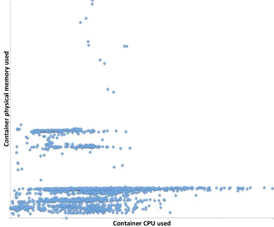
However, in a multi-tenant distributed system, different jobs and containers generally have widely different hardware usage profiles—some containers require significant memory, whereas some use CPU much more heavily (see Figure 2-1). Not considering CPU usage in scheduling meant that the system might be significantly underutilized, and some users would end up getting more or less than their true fair share of the cluster. A policy called Dominant Resource Fairness (DRF) addresses these limitations by considering multiple resource types and expressing the usage of each resource in a common currency (the share of the total allocation of that resource), and then scheduling based on the resource each container is using most heavily.
Figure 2-1. Per-container physical memory usage versus CPU usage during a representative period of time on a production cluster. Note that some jobs consume large amounts of memory while using relatively little CPU; others use significant CPU but
relatively little memory.
In Hadoop, operators can configure both the Fair Scheduler and the Capacity Scheduler to consider both memory and CPU (using the DRF framework) when considering which container to launch next on a given node.
Aggressive Scheduling for Busy Queues
Often a multi-tenant cluster might be in a state where some but not all queues are full; that is, some tenants currently don’t have enough work to use their full share of the cluster, but others have more work than they are guaranteed based on the scheduler’s configured allocation. In such cases, the scheduler might launch more containers from the busy queues to keep the cluster fully utilized.
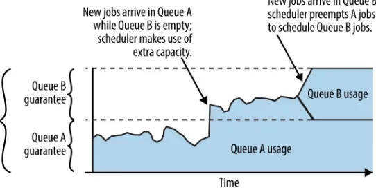
Sometimes, after those extra containers are launched, new jobs are submitted to a queue that was previously empty; based on the scheduler’s policy, containers from those jobs should be scheduled immediately, but because the scheduler has already opportunistically launched extra containers from other queues, the cluster is full. In those cases, the scheduler might preempt those extra containers by killing some of them in order to reflect the desired fairness policy (see Figure 2-2). Preemption is a common feature in schedulers for multi-tenant distributed systems, including both popular Hadoop schedulers (capacity and fair).
Because preemption inherently results in lost work, it’s important for the scheduler to strike a good balance between starting many opportunistic containers to make use of idle resources and avoiding too much preemption and the waste that it causes. To help reduce the negative impacts of preemption, the scheduler can slightly delay killing containers (to avoid wasting the work of containers that are almost complete) and generally chooses to kill containers that have recently launched (again, to avoid wasted work).
Figure 2-2. When new jobs arrive in Queue A, they might be scheduled if there is sufficient unused cluster capacity, allowing Queue A to use more than its guaranteed share. If jobs later arrive in Queue B, the scheduler might then preempt some of the
Queue A jobs to provide Queue B its guaranteed share.
A related concept is used by Google’s Borg system, which has a concept of priorities and quotas; a quota represents a set of hardware resource quantities (CPU, memory, disk, etc.) for a period of time, and higher-priority quota costs more than lower-priority quota. Borg never allocates more
production-priority quota than is available on a given cluster; this guarantees production jobs the resources they need. At any given time, excess resources that are not being used by production jobs can be used by lower-priority jobs, but those jobs can be killed if the production jobs’ usage later increases. (This behavior is similar to another kind of distributed system, Amazon Web Services, which has a concept of guaranteed instances and spot instances; spot instances cost much less than guaranteed ones but are subject to being killed at any time.)
Special Scheduling Treatment for Small Jobs
Some cluster operators provide special treatment for small or fast jobs; in a sense, this is the opposite of preemption. One example is LinkedIn’s “fast queue” for Hadoop, which is a small queue that is used only for jobs that take less than an hour total to run and whose containers each take less than 15 minutes. If jobs or containers violate this limit, they are automatically killed. This feature provides fast response for smaller jobs even when the cluster is bogged down by large batch jobs; it also encourages developers to optimize their jobs to run faster.
The Hadoop vendor MapR provides somewhat similar functionality with its ExpressLane, which schedules small jobs (as defined by having few containers, each with low memory usage and small input data sizes) to run on the cluster even when the cluster is busy and has no additional capacity for normal jobs. This is also an interesting example of using the input data size as a cue to the scheduler about how fast a container is likely to be.
Workload-Specific Scheduling Considerations
Aside from the general goals of high utilization and fairness across users and queues, schedulers
might take other factors into account when deciding which containers to launch and where to run them. For example, a key design point of Hadoop is to move computation to the data. (The goal is to not just get the nodes to work as hard as they can, but also get them to work more efficiently.) The scheduler tries to accomplish this goal by preferring to place a given container on one of the nodes that have the container’s input HDFS data stored locally; if that can’t be done within a certain amount of time, it then tries to place the container on the same rack as a node that has the HDFS data; if that also can’t be done after waiting a certain amount of time, the container is launched on any node that has
available computing resources. Although this approach increases overall system efficiency, it complicates the scheduling problem.
An example of a different kind of placement constraint is the support for pods in Kubernetes. A pod is a group of containers, such as Docker containers, that are scheduled at the same time on the same node. Pods are frequently used to provide services that act as helper programs for an application. Unlike the preference for data locality in Hadoop scheduling, the colocation and coscheduling of containers in a pod is a hard requirement; in many cases the application simply would not work without the auxiliary services running on the same node.
A weaker constraint than colocation is the concept of gang scheduling, in which an application requires all of its resources to run concurrently, but they don’t need to run on the same node. An example is a distributed database like Impala, which needs to have all of its “query fragments” running in order to serve queries. Although some distributed systems’ schedulers support gang scheduling natively, Hadoop doesn’t currently support gang scheduling; applications that require concurrent containers mimic gang scheduling by keeping containers alive but idle until all of the required containers are running. This workaround clearly wastes resources because these idle containers hold resources and stop other containers from running. However, even when gang
7
scheduling is done “cleanly” by the scheduler, it can lead to inefficiencies because the scheduler needs to avoid fully loading the cluster with other containers to ensure that enough space will eventually be available for the entire gang to be scheduled.
As a side note, workflow schedulers such as Oozie are given information about the dependencies among jobs in a complex workflow that must happen in order; the workflow scheduler then submits the individual jobs to the distributed system on behalf of the user. A workflow scheduler can take into account the required inputs and outputs of each stage (including inputs that depend on some off-cluster process to write new data to the cluster), the time of day the workflow should be started, awareness of the full directed acyclic graph (DAG) of the entire workflow, and similar constraints. Generally, the workflow scheduler is distinct from the distributed system’s own scheduler that determines exactly where and when containers are launched on each node, but there are cases when overall scheduling can be much more efficient if workflow scheduling and resource scheduling are combined.
Inefficiencies in Scheduling
Although schedulers have become more sophisticated over time, they continue to suffer from
inefficiencies related to the diversity of workloads running on multi-tenant distributed systems. These inefficiencies arise from the need to avoid overcommitting memory when doing up-front scheduling, a limited ability to consider all types of hardware resources, and challenges in considering the
dependencies among all jobs and containers within complicated workflows.
The Need to be Conservative with Memory
Distributed system schedulers generally make scheduling decisions based on conservative
assumptions about the hardware resources—especially memory—required by each container. These requirements are usually declared by the job author based on the worst-case usage, not the actual usage. This difference is critical because often different containers from the same job have different actual resource usage, even if they are running identical code. (This happens, for example, when the input data for one container is larger or otherwise different from the input data for other containers, resulting in a need for more processing or more space in memory.)
If a node’s resources are fully scheduled and the node is “unlucky” in the mix of containers it’s
running, the node can be overloaded; if the resource that is overloaded is memory, the node might run out of memory and crash or start swapping badly. In a large distributed system, some nodes are bound to be unlucky in this way, so if the scheduler does not use conservative resource usage estimates, the system will nearly always be in a bad state.
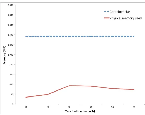
The need to be conservative with memory allocation means that most nodes will be underutilized most of the time; containers generally do not often use their theoretical maximum memory, and even when they do, it’s not for the full lifetime of the container (see Figure 2-3). (In some cases, containers can use even more than their declared maximum. Systems can be more or less stringent about
enforcing what the developer declares—some systems kill containers when they exceed their maximum memory, but others do not. )
Figure 2-3. Actual physical memory usage compared to the container size (the theoretical maximum) for a typical container. Note that the actual usage changes over time and is much smaller than the reserved amount.
To reduce the waste associated with this underutilization, operators of large multi-tenant distributed systems often must perform a balancing act, trying to increase cluster utilization without pushing nodes over the edge. As described in Chapter 4, software like Pepperdata provides a way to increase utilization for distributed systems such as Hadoop by monitoring actual physical memory usage and dynamically allowing more or fewer processes to be scheduled on a given node, based on the current and projected future memory usage on that node.
Inability to Effectively Schedule the Use of Other Resources
Similar inefficiencies can occur due to the natural variation over time in the resource usage for a single container, not just variation across containers. For a given container, memory usage tends to vary by a factor of two or three over the lifetime of the container, and the variation is generally smooth. CPU usage varies quite a bit over time, but the maximum usage is generally limited to a single core. In contrast, disk I/O and network usage frequently vary by orders of magnitude, and they
Figure 2-4. The variation over time in usage of different hardware resources for a typical MapReduce job. (source: Pepperdata)
Some schedulers (such as those in Hadoop) characterize computing nodes in a fairly basic way, allocating containers to a machine based on its total RAM and the number of cores. A more powerful scheduler would be aware of different hardware profiles (such as CPU speed and the number and type of hard drives) and match the workload to the right machine. (A somewhat related approach is budget-driven scheduling for heterogeneous clusters, where each node type might have both different hardware profiles and different costs. ) Similarly, although modern schedulers use DRF to help ensure fairness across jobs that have different resource usage characteristics, DRF does not optimize efficiency; an improved scheduler could use the cluster as a whole more efficiently by ensuring that each node has a mix of different types of workloads, such as CPU-heavy workloads running alongside data-intensive workloads that use much more disk I/O and memory. (This multidimensional packing problem is NP-hard, but simple heuristics could help performance significantly.)
Deadlock and Starvation
In some cases, schedulers might choose to start some containers in a job’s DAG even before the preceding containers (the dependencies) have completed. This is done to reduce the total run time of the job or spread out resource usage over time.
NOTE
In the interest of concreteness, the discussion in this section uses map and reduce containers, but similar effects can happen any time a job has some containers that depend on the output of others; the problems are not specific to MapReduce or Hadoop.
An example is Hadoop’s “slow start” feature, in which reduce containers might be launched before all of the map containers they depend on have completed. This behavior can help minimize spikes in network bandwidth usage by spreading out the heavy network traffic of transferring data from
mappers to reducers. However, starting a reduce container too early means that it might end up just sitting on a node waiting for its input data (from map containers) to be generated, which means that other containers are not able to use the memory the reduce container is holding, thus affecting overall system utilization.
This problem is especially common on very busy clusters with many tenants because often not all map containers from a job can be scheduled in quick succession; similarly, if a map container fails (for example, due to node failure), it might take a long time to get rescheduled, especially if other, higher-priority jobs have been submitted after the reducers from this job were scheduled. In extreme cases this can lead to deadlock, when the cluster is occupied by reduce containers that are unable to proceed because the containers they depend on cannot be scheduled. Even if deadlock does not occur, the cluster can still be utilized inefficiently, and overall job completion can be unnecessarily
11
12
13
slow as measured by wall-clock time, if the scheduler launches just a small number of containers from each of many users at one time.
A similar scheduling problem is starvation, which can occur on a heavily loaded cluster. For
example, consider a case in which one job has containers that each need a larger amount of memory than containers from other jobs. When one of the small containers completes on a node, a naive scheduler will see that the node has a small amount of memory available, but because it can’t fit one of the large containers there, it will schedule a small container to run. In the extreme case, the larger containers might never be scheduled. In Hadoop and other systems, the concept of a reservation
allows an application to reserve available space on a node, even if the application can’t immediately use it. (This behavior can help avoid starvation, but it also means that the overall utilization of the system is lower, because some amount of resources might be reserved but unused at any particular time.)
Waste Due to Speculative Execution
Operators can configure Hadoop to use speculative execution, in which the scheduler can observe that a given container seems to be running more slowly than is typical for that kind of container and start another copy of that container on another node. This behavior is primarily intended to avoid cases in which a particular node is performing badly (usually due to a hardware problem) and an entire job could be slowed down due to just one straggler container.
While speculative execution can reduce job completion time due to node problems, it wastes
resources when the container that is duplicated simply had more work to do than other containers and so naturally ran longer. In practice, experienced operators typically disable speculative execution on multi-tenant clusters, both because there is generally inherent container variation (not due to hardware problems) and because the operators are constantly watching for bad hardware, so speculative
execution does not enhance performance.
Summary
Over time, distributed system schedulers have grown in sophistication from a very simple FIFO algorithm to add the twin goals of fairness across users and increased cluster utilization. Those two goals must be balanced against each other; on multi-tenant distributed systems, operators often
prioritize fairness. They do so to reduce the level of user-visible scheduling issues as well as to keep multiple business units satisfied to use shared infrastructure rather than running their own separate clusters. (In contrast, configuring the scheduler to maximize utilization could save money in the short term but waste it in the long term, because many small clusters are less efficient than one large one.) Schedulers have also become more sophisticated by better taking into account multiple hardware resource requirements (for example, not considering only memory) and effectively treating different kinds of workloads differently when scheduling decisions are made. However, they still suffer from limitations, for example being conservative in resource allocation to avoid instability due to
15
overcommitting resources such as memory. That conservatism can keep the cluster stable, but it results in lower utilization and slower run times than the hardware could actually support. Software solutions that make real-time, fine-grained decisions about resource usage can provide increased utilization while maintaining cluster stability and providing more predictable job run times.
The new architecture is referred to as Yet Another Resource Negotiator (YARN) or MapReduce v2. See https://hadoop.apache.org/docs/r2.7.2/hadoop-yarn/hadoop-yarn-site/YARN.html.
See http://mesos.apache.org/api/latest/java/org/apache/mesos/Scheduler.html.
See https://www.quora.com/How-does-two-level-scheduling-work-in-Apache-Mesos.
Ghodsi, Ali, et al. “Dominant Resource Fairness: Fair Allocation of Multiple Resource Types.”
NSDI. Vol. 11. 2011. https://www.cs.berkeley.edu/~alig/papers/drf.pdf
See http://hadoop.apache.org/docs/current/hadoop-yarn/hadoop-yarn-site/FairScheduler.html
and http://hadoop.apache.org/docs/current/hadoop-yarn/hadoop-yarn-site/CapacityScheduler.html.
Verma, Abhishek, et al. “Large-scale cluster management at Google with Borg.” Proceedings of the Tenth European Conference on Computer Systems. ACM, 2015.
http://research.google.com/pubs/archive/43438.pdf
See slide 9 of http://www.slideshare.net/Hadoop_Summit/hadoop-operations-at-linkedin. See http://doc.mapr.com/display/MapR/ExpressLane.
Nurmi, Daniel, et al. “Evaluation of a workflow scheduler using integrated performance modelling and batch queue wait time prediction.” Proceedings of the 2006 ACM/IEEE conference on
Supercomputing. ACM, 2006. http://www.cs.ucsb.edu/~nurmi/nurmi_workflow.pdf
For example, Google’s Borg kills containers that try to exceed their declared memory limit. Hadoop by default lets containers go over, but operators can configure it to kill such containers.
Wang, Yang and Wei Shi. “Budget-driven scheduling algorithms for batches of MapReduce jobs in heterogeneous clouds.” IEEE Transactions on Cloud Computing 2.3 (2014): 306-319.
https://www.researchgate.net/publication/277583513_Budget-Driven-Scheduling-Algorithms-for-Batches-of-MapReduce-Jobs
See, for example, Chekuri, Chandra and Sanjeev Khanna. “On multidimensional packing problems.” SIAM journal on computing 33.4 (2004): 837-851.
http://repository.upenn.edu/cgi/viewcontent.cgi?article=1080&context=cis_papers
See http://stackoverflow.com/questions/11672676/when-do-reduce-tasks-start-in-hadoop/11673808#11673808.
See https://issues.apache.org/jira/browse/MAPREDUCE-314 for an example.
See Sulistio, Anthony, Wolfram Schiffmann, and Rajkumar Buyya. “Advanced reservation-based
scheduling of task graphs on clusters.” International Conference on High-Performance Computing. Springer Berlin Heidelberg, 2006. http://www.cloudbus.org/papers/workflow_hipc2006.pdf. For related recent work in Hadoop, see Curino, Carlo et al. “Reservation-based Scheduling: If You’re Late Don’t Blame Us!” Proceedings of the ACM Symposium on Cloud Computing. ACM, 2014.
https://www.microsoft.com/en-us/research/publication/reservation-based-scheduling-if-youre-late-dont-blame-us/.
This is different from the standard use of the term “speculative execution” in which pipelined microprocessors sometimes execute both sides of a conditional branch before knowing which branch will be taken.
Chapter 3. CPU Performance
Considerations
Introduction
Historically, large-scale distributed systems were designed to perform massive amounts of numerical computation, for example in scientific simulations run on high-performance computing (HPC)
platforms. In most cases, the work done on such systems was extremely compute intensive, so the CPU was often the primary bottleneck.
Today, distributed systems tend to run applications for which the large scale is driven by the size of the input data rather than the amount of computation needed—examples include both special-purpose distributed systems (such as those powering web search among billions of documents) and general-purpose systems such as Hadoop. (However, even in those general systems, there are still some cases such as iterative algorithms for machine learning where making efficient use of the CPU is critical.) As a result, the CPU is often not the primary bottleneck limiting a distributed system; nevertheless, it is important to be aware of the impacts of CPU on overall speed and throughput.
At a high level, the effect of CPU performance on distributed systems is driven by three primary factors:
The efficiency of the program that’s running, at the level of the code as well as how the work is broken into pieces and distributed across nodes.
Low-level kernel scheduling and prioritization of the computational work done by the CPU, when the CPU is not waiting for data.
The amount of time the CPU spends waiting for data from memory, disk, or network.
These factors are important for the performance even of single applications running on a single machine; they are just as important, and even more complicated, for multi-tenant distributed systems due to the increased number and diversity of processes running on those systems, and their varied input data sources.
Algorithm Efficiency
Of course, as with any program, when writing a distributed application, it is important to select a good algorithm (such as implementing algorithms with N*log(N) complexity instead of N , using joins efficiently, etc.) and to write good code; the best way to spend less time on the CPU is to avoid
computation in the first place. As with any computer program, developers can use standard
performance optimization and profiling tools (open source options include gprof, hprof, VisualVM,
and Perf4J; Dynatrace is one commercial option) to profile and optimize a single instance of a program running on a particular machine.
For distributed systems, it can be equally important (if not more so) to break down the work into units effectively. For example, with MapReduce programs, some arrangements of map-shuffle-reduce steps are more efficient than others. Likewise, whether using MapReduce, Spark, or another distributed framework, using the right level of parallelism is important. For example, because every map and reduce task requires a nontrivial amount of setup and teardown work, running too many small tasks can lead to grossly inefficient overhead—we’ve seen systems with thousands of map tasks that each require several seconds for setup and teardown but spend less than one second on useful computation. In the case of Hadoop, open source tools like Dr. Elephant (as well as some commercial tools)
provide performance measurement and recommendations to improve the overall flow of jobs, identifying problems such as a suboptimal breakdown of work into individual units.
Kernel Scheduling
The operating system kernel (Linux, for example) decides which threads run where and when,
distributing a fixed amount of CPU resource across threads (and thus ultimately across applications). Every N (~5) milliseconds, the kernel takes control of a given core and decides which thread’s
instructions will run there for the next N milliseconds. For each candidate thread, the kernel’s scheduler must consider several factors:
Is the thread ready to do anything at all (versus waiting for I/O)? If yes, is it ready to do something on this core?
If yes, what is its dynamic priority? This computation takes several factors into account, including the static priority of the process, how much CPU time the thread has been allocated recently, and other signals depending on the kernel version.
How does this thread’s dynamic priority compare to that of other threads that could be run now? The Linux kernel exposes several control knobs to affect the static (a priori) priority of a process; nice and control groups (cgroups) are the most commonly used. With cgroups, priorities can be set, and scheduling affected, for a group of processes rather than a single process or thread; conceptually, cgroups divide the access to CPU across the entire group. This division across groups of processes means that applications running many processes on a node do not receive unfair advantage over applications with just one or a few processes.
In considering the impact of CPU usage, it is helpful to distinguish between latency-sensitive and
latency-insensitive applications:
In a latency-sensitive application, a key consideration is the timing of the CPU cycles assigned to it. Performance can be defined by the question “How much CPU do I get when I need it?”
In a latency-insensitive application, the opposite situation exists: the exact timing of the CPU cycles assigned to it is unimportant; the most important consideration is the total number of CPU cycles assigned to it over time (usually minutes or hours).
This distinction is important for distributed systems, which often run latency-sensitive applications alongside batch workloads, such as MapReduce in the case of Hadoop. Examples of latency-sensitive distributed applications include search engines, key-value stores, clustered databases, video
streaming systems, and advertising systems with real-time bidding that must respond in milliseconds. Examples of latency-insensitive distributed applications include index generation and loading for search engines, garbage collection for key-value stores or databases, and offline machine learning for advertising systems.
An interesting point is that even the same binary can have very different requirements when used in different applications. For example, a distributed data store like HBase can be latency-sensitive for reading data when serving end-customer queries, and latency-insensitive when updating the
underlying data—or it can be latency-sensitive for writing data streamed from consumer devices, and latency-insensitive when supporting analyst queries against the stored data. The semantics of the specific application matter when setting priorities and measuring performance.
Intentional or Accidental Bad Actors
As is the case with other hardware resources, CPU is subject to either intentional or accidental “bad actors” who can use more than their fair share of the CPU on a node or even the distributed system as a whole. These problems are specific to multi-tenant distributed systems, not single-node systems or distributed systems running a single application.
A common problem case is due to multithreading. If most applications running in a system are single threaded, but one developer writes a multithreaded application, the system might not be tuned
appropriately to handle the new type of workload. Not only can this cause general performance
problems, it is considered unfair because that one developer can nearly monopolize the system. Some systems like Hadoop try to mitigate this problem by allowing developers to specify how many cores each task will use (with multithreaded programs specifying multiple cores), but this can be wasteful of resources, because if a task is not fully using the specified number of cores, the cores might remain reserved and thus go unused.
Applying the Control Mechanisms in Multi-Tenant Distributed Systems
Over time, kernel mechanisms have added additional knobs like cgroups and CPU pinning, but today there is still no general end-to-end system that makes those mechanisms practical to use. For example, there is no established policy mechanism to require applications to state their need, and no distributed system framework connects application policies with kernel-level primitives.
running there. Getting things to run smoothly requires the administrator to have a good “feel” for the way the cluster normally behaves, and to watch and tune it constantly.
In some special cases, software developers have designed their platforms so that they can use CPU priorities to affect overall application performance. For example, the Teradata architecture was designed to make all queries CPU bound, and then CPU priorities can be used to control overall query prioritization and performance. Similarly, HPC frameworks like Portable Batch System (PBS) and Terascale Open-Source Resource and QUEue Manager (TORQUE) support cgroups.
For general-purpose, multi-tenant distributed systems like Hadoop, making effective use of kernel primitives such as cgroups is more difficult, because a given system might be running a multitude of diverse workloads at any given time. Even if CPU were the only limited resource, it would be difficult to adjust the settings correctly in such an environment, because the amount of CPU required by the various applications changes constantly. Accounting for RAM, disk I/O, and network only multiplies the complexity. Further complicating the situation is the fact that distributed systems
necessarily divide applications into tens, hundreds, or thousands of processes across many nodes, and giving one particular process a higher priority might not affect the run time of the overall application in a predictable way.
Software such as Pepperdata helps address these complications and other limitations of Hadoop. With Pepperdata, Hadoop administrators set high-level priorities for individual applications and groups of applications, and Pepperdata constantly monitors each process’s use of hardware and responds in real time to enforce those priorities, adjusting kernel primitives like nice and cgroups.
I/O Waiting and CPU Cache Impacts
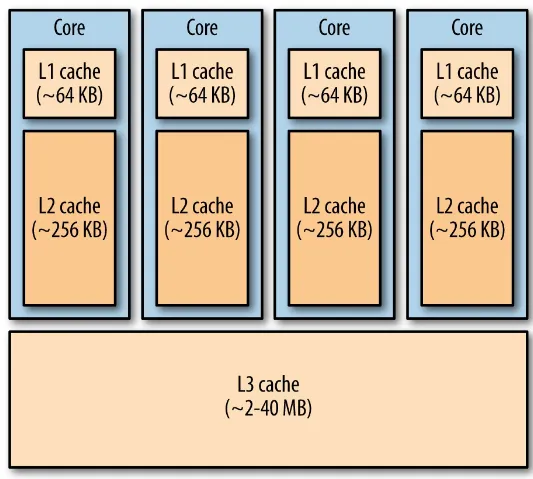
The performance impact of waiting for disk and network I/O on multi-tenant distributed systems is covered in Chapters 4 and 5 of this book; this section focuses on the behavior of the CPU cache. In modern systems, CPU chip speeds are orders of magnitude faster than memory speeds, so
Figure 3-1. Typical cache architecture for a multicore CPU chip.
Well-designed programs that are predominantly running alone on one or more cores can often make very effective use of the L1/L2/L3 caches and thus spend most of their CPU time performing useful computation. In contrast, multi-tenant distributed systems are an inherently more chaotic environment, with many processes running on the same machine and often on the same core. In such a situation, each time a different process runs on a core, the data it needs might not be in the cache, so it must wait for data to come from main memory—and then when it does, that new data replaces what was previously in the cache, so when the CPU switches back to a process it had already been running, that process, in turn, must fetch its data from main memory. These pathological cache misses can cause most of the CPU time to be wasted waiting for data instead of processing it. (Such situations can be difficult to detect because memory access/wait times show up in most metrics as CPU time.)
machine can slow things down because the kernel must spend a lot of CPU time engaged in context switching. (This excessive kernel overhead can be seen in kernel metrics such as
voluntary_ctxt_switches and nonvoluntary_ctxt_switches via the /proc filesystem, or by using a tool such as SystemTap.)
The nature of multi-tenant systems also exacerbates the cache miss problem because no single developer or operator is tuning and shaping the processes within the box—a single developer therefore has no control over what else is running on the box, and the environment is constantly changing as new workloads come and go. In contrast, special-purpose systems (even distributed ones) can be designed and tuned to minimize the impact of cache misses and similar performance problems. For example, in a web-scale search engine, each user query needs the system to process different data to produce the search results. A naive implementation would distribute queries
randomly across the cluster, resulting in high cache miss rates, with the CPU cache constantly being overwritten. Search engine developers can avoid this problem by assigning particular queries to subsets of the cluster. This kind of careful design and tuning is not possible with general-purpose, multi-tenant distributed systems.
Similarly, another aspect of distributed systems can affect developers’ mindsets: because they have access to much more RAM than they would on a single computer, they might naturally begin to think of RAM as an elastic resource that incurs no performance penalty when accessed. They might thus pay less attention to the details of hardware usage and its performance implications than they otherwise would.
Summary
CPU utilization is a key metric for improving the performance of a distributed system. If CPU utilization is high for the distributed system (overall or on one particular “hotspot” node), it is
important to determine whether that CPU utilization reflects useful work (the computation required by the application) or waste due to overhead, such as task startup/teardown, context switching, or CPU cache misses.
Developers can reduce this overhead in some straightforward ways, such as optimizing the division of an application into discrete units. In addition, operators should use tools to control CPU priorities so that CPU cycles are dedicated to the most important workloads when they need them.
See https://github.com/linkedin/dr-elephant/wiki.
Typically 64-256 KB for the L1 and L2 cache for each core, and a few megabytes for the L3 cache that is shared across cores; see https://en.wikipedia.org/wiki/Haswell_%28microarchitecture%29.
See http://blog.tsunanet.net/2010/11/how-long-does-it-take-to-make-context.html for interesting data on context switch times.
3
1 2
Chapter 4. Memory Usage in Distributed
Systems
Introduction
Memory is fundamentally different from other hardware resources (CPU, disk I/O, and network) because of its behavior over time: when a process accesses a certain amount of memory, the process generally keeps and holds that memory even if it is not being used, until the process completes. In this sense, memory behaves like a ratchet (a process’s memory usage increases or stays constant over time but rarely decreases) and is not time-shiftable.
Also unlike other hardware resources (for which trying to use more than the node’s capacity merely slows things down), trying to use more than the physical memory on the node can cause it to
misbehave badly, in some cases with arbitrary processes being killed or the entire node freezing up and requiring a physical reboot.
Physical Versus Virtual Memory
Modern operating systems use virtual memory to conceptually provide more memory to applications than is physically available on the node. The operating system (OS) exposes to each process a virtual memory address that maps to a physical memory address, dividing the virtual memory space into
pages of 4 KB or more. If a process needs to access a virtual memory address whose page is not currently in physical memory, that page is swapped in from a swap file on disk. When the physical memory is full, and a process needs to access memory that is not currently in physical memory, the OS selects some pages to swap out to disk, freeing up physical memory.
Many modern languages such as Java perform memory management via garbage collection, but one side effect of doing so is that garbage collection itself touches those pages in memory, so they will not be swapped out. Most multi-tenant distributed systems run applications written in a variety of
languages, and some of those applications will likely be doing garbage collection at any time, causing a reduction in swapping (and thus more physical memory usage).
A node’s virtual memory space can be much larger than physical memory for two primary reasons: A process requires a large amount of (virtual) memory, but it doesn’t need to use that much physical memory if it doesn’t access a particular page.
Because of swapping, some virtual memory is in physical memory, but some might be on disk.
In most cases, allowing the applications running on a node to use significantly more virtual memory than physical memory is not problematic. However, if many pages are being swapped in and out frequently, the node can begin thrashing, with most of the time on the node spent simply swapping pages in and out. (Keep in mind that disk seeks are measured in milliseconds, whereas CPU cycles and RAM access times are measured in nanoseconds, roughly a million times faster.)
Thrashing has two primary causes: Excessive oversubscription of memory
This results from running multiple processes, the sum of whose virtual memory is greater than the physical memory on the node. Generally, some oversubscription of memory is desired for
maximum utilization, as described later in this chapter. However, if there is too much oversubscription, and the running processes use significantly more virtual memory than the
physical memory on the node, the node can spend most of its time inefficiently swapping pages in and out as different processes are scheduled on the CPU. This is the most common cause of
thrashing.
NOTE
Although in most cases excess oversubscription is caused by the scheduler underestimating how much memory the set of processes on a node will require, in some cases a badly behaved application can cause this problem. For example, in some earlier versions of Hadoop, tasks could start other processes running on the node (using “Hadoop streaming”) that could use up much more memory than the tasks were supposed to.
An individual process might be too large for the machine
In some cases, the process’s working set (the amount of data that needs to be held in memory in order for the algorithm to work efficiently) is larger than the physical RAM on the node. In this case, either the application must be changed (to a different algorithm that uses memory differently, or by partitioning the application into more tasks to reduce the dataset size) or more physical memory must be added to the box.
As with many other issues described in this book, these problems can be exacerbated on multi-tenant distributed systems, for which a single node typically runs many processes from different workloads with different behaviors, and no one developer has the incentive or ability to tune a particular
application. (However, multi-tenant systems also provide possibilities for improved efficiency; for example, by running a memory-light but CPU-intensive application alongside an application that is a heavy user of memory.)
Detecting and Avoiding Thrashing
example, a node that is thrashing (as opposed to swapping in a healthy way) might exhibit the following symptoms:
Kernel metrics related to swapping show a significant amount of swapping in and out at the same time.
The amount of physical memory used is a very high fraction (perhaps 90 percent or more) of the memory on the node.
The node appears unresponsive or quite slow; for example, logging into the node takes 10–60 seconds instead of half a second, and when typing in a terminal an operator might see a delay before each character appears. Ultimately, the node can crash.
Because the node is so slow and unresponsive, logging in to try to fix things can become impossible. Even the system’s kernel processes that are trying to fix the problem might not be able to get enough resources to run.
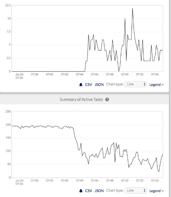
When a node begins thrashing badly, it is often too late to fix without physically power-cycling the node, so it is better to avoid thrashing altogether. A conservative approach would be to avoid
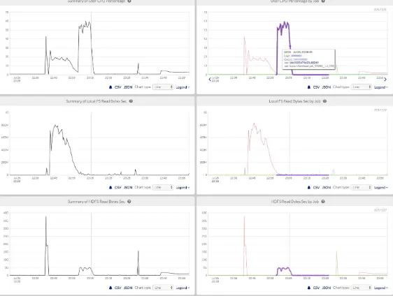
Figure 4-1. Detection of sudden, extreme swapping based on machine learning (top), and an automated response of stopping containers to maintain cluster stability (bottom). (source: Pepperdata)
Kernel Out-Of-Memory Killer
The Linux kernel has an out-of-memory (OOM) killer that steps in to free up memory when all else fails. If a node has more pages accessed by the sum of the processes on the node than the sum of physical memory and on-disk virtual memory, there’s no memory left, and the kernel’s only choice is to kill something. This frequently happens when on-disk swap space is set to be small or zero.
Unfortunately, from the point of view of applications running on the node, the kernel’s algorithm can appear random. The kernel is unaware of any semantics of the applications running on the node, so its choice of processes to kill might have unwanted consequences, such as the following:
Processes that have been running for a very long time and that are nearly complete, instead of newly-started processes for which little work would be wasted.
Processes that parts of a job running on other nodes depend on, such as tasks that are part of a larger workflow.
Underlying daemons of the distributed system (for example, the distributed file system process running on a node), whose killing can cause many jobs to stall, thus slowing down the entire distributed system.
Implications of Memory-Intensive Workloads for
Multi-Tenant Distributed Systems
As with other hardware resources, the impact of memory usage on multi-tenant distributed systems is more complicated than on a single node. This is because memory-intensive workloads run on many nodes in the cluster simultaneously, and processes running on different nodes in the cluster are interdependent. Both factors often can cause problems to cascade across the entire cluster. This problem is particularly bad with memory because unlike CPU, disk I/O, and network, for which bottlenecks only slow down a node or the cluster, memory limits that lead to thrashing or OOM killing can cause nodes and processes to go completely offline.
An example in the case of Hadoop is HDFS, in which data is replicated on a subset (usually three) of the nodes in the cluster, and running applications can access any one of the three replications. The scheduler can very easily cause memory-intensive workloads to run on many nodes of the cluster, resulting in thrashing or OOM killing occurring on many nodes at once. Those nodes might effectively freeze up due to thrashing, or the OOM killer might kill the daemon serving the HDFS data that is stored on the node. Losing access to just one replica of HDFS data can slow down processes running on other nodes on the cluster; for cases in which all three replicas of a certain file are on nodes where HDFS is unresponsive, jobs cannot run at all, and the entire cluster can grind to a halt.
Solutions
memory (e.g., a database query planner can calculate how much memory a query will take, and the database can wait to run that query until sufficient memory is available). Similarly, in a
high-performance computing (HPC) system dedicated to a specific workload, developers generally tune the workload’s memory usage carefully to match the physical memory of the hardware on which it will run. (In multi-tenant HPC, when applications start running, the state of the cluster cannot be known in advance, so such systems have memory usage challenges similar to systems like Hadoop.) In the general case, developers and system designers/operators can take steps to use memory more efficiently, such as the following:
For long-running applications (such as a distributed database or key-value store), a process might be holding onto memory that is no longer needed. In such a case, restarting the process on the node can free up memory immediately, because the process will come back up in a “clean” state. This kind of approach can work when the operator knows that it’s safe to restart the process; for
example, if the application is running behind a load balancer, one process can be safely restarted (on one node) at a time.
Some distributed computing fabrics like VMware’s vSphere allow operators to move virtual machines from one physical machine to another while running, without losing work. Operators can use this functionality to improve the efficiency and utilization of the distributed system as a whole by moving work to nodes that can better fit that work.
An application can accept external input into how much memory it should use and change its behavior as a result. For example, the application can use less cache or compress the data stored in memory, both of which trade more CPU time for less memory usage. This is similar to how the Linux kernel adjusts to use less disk cache space if running processes need more memory. An example of a specific application with this behavior is Oracle’s database, which compresses data in memory.
Hadoop tends to be very conservative in memory allocations; it generally assumes the worst case, that every process will require its full requested virtual memory for the entire run time of the process. This conservatism generally results in the cluster being dramatically underutilized because these two assumptions are usually untrue. As a result, even if a developer has tried to carefully tune the memory settings of a given job, most nodes will still have unused memory, due to several factors:
For a given process, the memory usage changes during its run time. (The usage pattern depends on the type of work the process is doing; for example, in the case of Hadoop, mappers tend to rapidly plateau, whereas reducers sometimes plateau and sometimes vary over time. Spark generally varies over time.)
Different parts of a job often vary in memory usage because they are working on different parts of the input data on different nodes.
A naive approach to improving cluster utilization by simply increasing memory oversubscription can often be counterproductive because the processes running on a node do sometimes use more memory than the physical memory available on the node. When that happens, the throughput of the node can decrease due to the inefficiency of excessive swapping, and if the node begins thrashing, it can have side effects on other nodes as well, as described earlier.
Software like Pepperdata provides a way to increase utilization for distributed systems such as Hadoop by monitoring actual physical memory usage and dynamically allowing more or fewer processes to be scheduled on a given node, based on the current and projected future memory usage on that node. These solutions can dramatically increase throughput while avoiding the negative consequences of overusing physical memory and the cascading failures that can result.
Summary
Memory is often the primary resource limiting the overall processing capacity of a node or an entire distributed system; it is common to see a system’s CPU, disk, and network running below capacity because of either actually or artificially limited memory use. At the opposite extreme,
Chapter 5. Disk Performance: Identifying
and Eliminating Bottlenecks
Introduction
Distributed systems frequently use a distributed file system (DFS). Today, such systems most
commonly store data on the disks of the compute nodes themselves, as in the Hadoop Distributed File System (HDFS). HDFS generally splits data files into large blocks (typically 128 MB) and then replicates each block on three different nodes for redundancy and performance.
Some systems (including some deployments of Hadoop) do not store the distributed file system data directly on the compute nodes and instead rely on cloud data storage (e.g., using Amazon’s S3 as storage for Hadoop and others) or network-attached storage (NAS). Even in these cases, some data is often copied to a compute node’s local disks before processing, or jobs’ intermediate or final output data might be written temporarily to the compute node’s local disks.
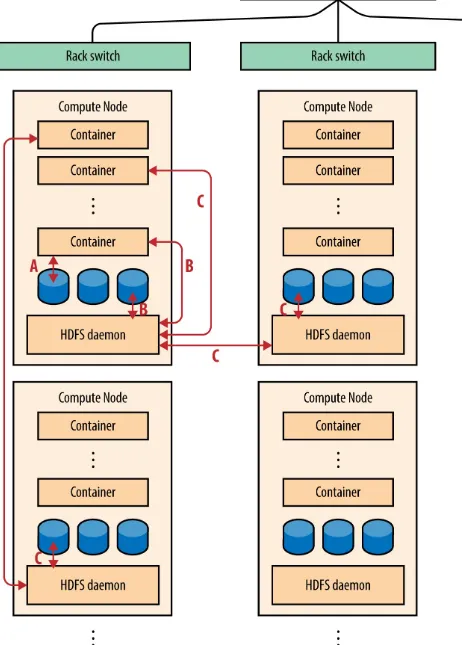
Whether using a system like HDFS that stores all of its data on the computing cluster itself or a system that uses separate storage such as S3 or NAS, there are three major conceptual locations of data (see
Figure 5-1): Truly local
Data is written to temporary files (such as spill files that cache local process output before being sent to remote nodes), log files, and so on.
Local but managed via the DFS
The data being read by a process on a node lives in HDFS, but the actual bytes are on a local disk on that node. (Hadoop tries to lay out computation to increase the likelihood that processes will use local data in this way.)
Remote
Figure 5-1. Locations of data in a distributed system that uses HDFS for storage. A: truly local disk access. B: Access to HDFS data stored on the local node. C: Access to HDFS data stored on another node, either on the same network rack or on another
network rack.
transform, and load [ETL] to/from some external source). Correspondingly, some disk performance impacts are due to local processes, and some are due to remote processes.
Overview of Disk Performance Limits
A single physical hard drive has two fundamental performance limits: Disk seek time
The amount of time it takes for the read/write head to move to a new track on the disk to access specific data. This time is typically a few milliseconds. (There is additional rotational latency
in waiting for the disk to spin until the desired data is under the head; this time is about half of the seek time.) The number of such disk operations is measured in I/O operations per second (IOPS). Disk throughput
The speed with which data can be read from or written to the disk after the head has moved to the desired track. Modern disks typically have sustained throughput of roughly 200 MBps. (Disk throughput is sometimes also referred to as disk bandwidth.)
A given disk becomes a bottleneck when the processes on the node are either trying to read or write data faster than the disk head or the disk controller can handle and thus have reached the throughput cap, or are reading or writing a large number of small files (rather than a few large files that are read sequentially from the disk) and thus causing too many seeks. The latter case is often due to the “small-files problem,” in which poorly-designed applications have broken their input or output data into too many small chunks. The end result of the small-files problem is that a disk that could otherwise read 200 MBps ends up only reading at a small fraction of that speed.
Disk Behavior When Using Multiple Disks
Modern servers have several hard drives per node, which generally improves performance. Striping disk reads and writes across multiple disks (which can be done either explicitly by the application, as in HDFS, or at a low level, as in RAID 0) generally increases both the total disk throughput and total IOPS of a node. For example, Hadoop spreads some intermediate temporary files (such as spills from mappers and inputs to reducers that come from the shuffle stage) across disks. Likewise, it’s a good practice to spread frequently flushed log files across disks because they are generally appended in very small pieces and writing/flushing them can cause many IOPS. Splitting the throughput and IOPS across many disks means that the CPU can spend more time doing useful work and less time waiting for input data.
However, if a particular disk is slow (due to hardware problems) or is being accessed more than the other disks on the node, that disk can effectively slow down the entire system; if a process must complete reading from or writing to files that are spread across all disks, its performance is
constrained by the slowest disk. This can happen, for example, if a particular HDFS file is located on