Structural Dynamics, Dynamic Force and Dynamic System
Structural Dynamics
Conventional structural analysis is based on the concept of statics, which can be derived from Newton’s
1st law of motion. This law states that it is necessary for some force to act in order to initiate motion of a body at rest or to change the velocity of a moving body. Conventional structural analysis considers the external forces or joint displacements to be static and resisted only by the stiffness of the structure. Therefore, the resulting displacements and forces resulting from structural analysis do not vary with time.
Structural Dynamics is an extension of the conventional static structural analysis. It is the study of structural analysis that considers the external loads or displacements to vary with time and the structure to
respond to them by its stiffness as well as inertia and damping. Newton’s 2nd
law of motion forms the basic principle of Structural Dynamics. This law states that the resultant force on a body is equal to its mass times the acceleration induced. Therefore, just as the 1st law of motion is a special case of the 2nd law, static structural analysis is also a special case of Structural Dynamics.
Although much less used by practicing engineers than conventional structural analysis, the use of Structural Dynamics has gradually increased with worldwide acceptance of its importance. At present, it is being used for the analysis of tall buildings, bridges, towers due to wind, earthquake, and for marine/offshore structures subjected wave, current, wind forces, vortex etc.
Dynamic Force
The time-varying loads are called dynamic loads. Structural dead loads and live loads have the same magnitude and direction throughout their application and are thus static loads. However there are several examples of forces that vary with time, such as those caused by wind, vortex, water wave, vehicle, impact, blast or ground motion like earthquake.
Dynamic System
A dynamic system is a simple representation of physical systems and is modeled by mass, damping and stiffness. Stiffness is the resistance it provides to deformations, mass is the matter it contains and damping represents its ability to decrease its own motion with time.
Mass is a fundamental property of matter and is present in all physical systems. This is simply the weight of the structure divided by the acceleration due to gravity. Mass contributes an inertia force (equal to mass times acceleration) in the dynamic equation of motion.
Stiffness makes the structure more rigid, lessens the dynamic effects and makes it more dependent on static forces and displacements. Usually, structural systems are made stiffer by increasing the cross-sectional dimension, making the structures shorter or using stiffer materials.
Free Vibration of Undamped Single-Degree-of-Freedom (SDOF) System
Formulation of the Single-Degree-of-Freedom (SDOF) Equation
A dynamic system resists external forces by a combination of forces due to its stiffness (spring force), damping (viscous force) and mass (inertia force). For the system shown in Fig. 2.1, k is the stiffness, c the viscous damping, m the mass and u(t) is the dynamic displacement due to the time-varying excitation force f(t). Such systems are called Single-Degree-of-Freedom (SDOF) systems because they have only one dynamic displacement [u(t) here].
m f(t), u(t) f(t)
k c
Fig. 2.1: Dynamic SDOF system subjected to dynamic force f(t)
Considering the free body diagram of the system, f(t) fS fV = ma …………..(2.1)
where fS = Spring force = Stiffness times the displacement = k u …..………(2.2)
fV = Viscous force = Viscous damping times the velocity = c du/dt …..………(2.3)
fI = Inertia force = Mass times the acceleration = m d 2
u/dt2 ..…………(2.4)
Combining the equations (2.2)-(2.4) with (2.1), the equation of motion for a SDOF system is derived as,
m d2u/dt2 + c du/dt + ku = f(t) …..………(2.5)
This is a 2nd order ordinary differential equation (ODE), which needs to be solved in order to obtain the dynamic displacement u(t). As will be shown subsequently, this can be done analytically or numerically.
Eq. (2.5) has several limitations; e.g., it is assumed on linear input-output relationship [constant spring (k) and dashpot (c)]. It is only a special case of the more general equation (2.1), which is an equilibrium equation and is valid for linear or nonlinear systems. Despite these, Eq. (2.5) has wide applications in Structural Dynamics. Several important derivations and conclusions in this field have been based on it.
Free Vibration of Undamped Systems
Free Vibration is the dynamic motion of a system without the application of external force; i.e., due to initial excitement causing displacement and velocity.
The equation of motion of a general dynamic system with m, c and k is,
m d2u/dt2 + c du/dt + ku = f(t) …..………(2.5)
For free vibration, f(t) = 0; i.e., m d2u/dt2 + c du/dt + ku = 0
For undamped free vibration, c = 0 m d2u/dt2 + ku = 0 d2u/dt2 + n 2
u = 0 ..…………(2.6)
where n = (k/m), is called the natural frequency of the system ..…………(2.7)
Assume u = est, d2u/dt2 = s2est s2 est + n 2
est = 0 s = i n .
u (t) = Aei n t + B e-i n t = C1 cos ( nt) + C2 sin ( nt) …..………(2.8)
v (t) = du/dt = -C1 n sin ( nt) + C2 n cos ( nt) ....……..…(2.9)
If u(0) = u0 and v(0) = v0, then C1 = u0 and C2 n = v0 C2 = v0/ n ……..…..(2.10)
u(t) = u0 cos ( nt) + (v0/ n) sin ( nt) …...…….(2.11)
fS fV
Natural Frequency and Natural Period of Vibration
Eq (2.11) implies that the system vibrates indefinitely with the same amplitude at a frequency of n
radian/sec. Here, n is the angular rotation (radians) traversed by a dynamic system in unit time (one
second). It is called the natural frequencyof the system (in radians/sec).
Alternatively, the number of cycles completed by a dynamic system in one second is also called its
natural frequency (in cycles/sec or Hertz). It is often denoted by fn. fn = n/2 …………(2.12)
The time taken by a dynamic system to complete one cycle of revolution is called its natural period (Tn).
It is the inverse of natural frequency.
Tn = 1/fn = 2 / n …………..(2.13)
Example 2.1
An undamped structural system with stiffness (k) = 25 k/ft and mass (m) = 1 k-sec2/ft is subjected to an initial displacement (u0) = 1 ft and an initial velocity (v0) = 4 ft/sec.
(i) Calculate the natural frequency and natural period of the system. (ii) Plot the free vibration of the system vs. time.
Solution
(i) For the system, natural frequency, n = (k/m) = (25/1) = 5 radian/sec
fn = n/2 = 5/2 = 0.796 cycle/sec
Natural period, Tn = 1/fn = 1.257 sec
(ii) The free vibration of the system is given by Eq (2.11) as
u(t) = u0 cos ( nt) + (v0/ n) sin ( nt) = (1) cos (5t) + (4/5) sin (5t) = (1) cos (5t) + (0.8) sin (5t)
The maximum value of u(t) is = (12 + 0.82) = 1.281 ft. The plot of u(t) vs. t is shown below in Fig. 2.2.
Fig. 3.1: Displacement vs. Time for free vibration of an undamped system -1.5
-1 -0.5 0 0.5 1 1.5
0 1 2 3 4 5
Time (sec)
D
is
p
la
c
e
m
e
n
t
(ft
)
Free Vibration of Damped Systems
As mentioned in the previous section, the equation of motion of a dynamic system with mass (m), linear viscous damping (c) & stiffness (k) undergoing free vibration is,
m d2u/dt2 + c du/dt + ku = 0 .………(2.5)
1. If 1, the system is called an overdamped system. Here, the solution for s is a pair of different real
numbers [ n( + (
2
1)), n( (
2
1))]. Such systems, however, are not very common. The displacement u(t) for such a system is
u(t) = e- n t (Ae 1 t + B e- 1 t) ……….………….(3.4)
where 1 = n ( 2
1)
2. If = 1, the system is called a critically damped system. Here, the solution for s is a pair of identical real numbers [ n, n]. Critically damped systems are rare and mainly of academic interest only.
The displacement u(t) for such a system is
u(t) = e n t (A + Bt) ….……….(3.5) The displacement u(t) for such a system is
u(t) = e nt (Aei d t + B e-i d t) = e nt [C1 cos ( dt) + C2 sin ( dt)] …...………(3.6)
where d = n (1 2
) is called the damped natural frequency of the system.
Since underdamped systems are the most common of all structural systems, the subsequent discussion will focus mainly on those. Differentiating Eq (3.6), the velocity of an underdamped system is obtained as
v(t) = du/dt
decreases steadily, and reaches zero after (a hypothetical) ‘infinite’ time of vibration.
Example 3.1
A damped structural system with stiffness (k) = 25 k/ft and mass (m) = 1 k-sec2/ft is subjected to an initial displacement (u0) = 1ft and an initial velocity (v0) = 4 ft/sec. Plot the free vibration of the system vs. time
if the Damping Ratio ( ) is
(a) 0.00 (undamped system),
(b) 0.05, (c) 0.50 (underdamped systems), (d) 1.00 (critically damped system), (e) 1.50 (overdamped system).
Solution
The equations for u(t) are plotted against time for various damping ratios (DR) and shown below in Fig. 3.1. The main features of these figures are
(1) The underdamped systems have sinusoidal variations of displacement with time. Their natural periods are lengthened (more apparent for = 0.50) and maximum amplitudes of vibration reduced due to damping.
(2) The critically damped and overdamped systems have monotonic rather than harmonic (sinusoidal) variations of displacement with time. Their maximum amplitudes of vibration are less than the amplitudes of underdamped systems.
Fig. 4.1: Displacement vs. Time for free vibration of damped systems -1.5
-1 -0.5 0 0.5 1 1.5
0 1 2 3 4 5
Time (sec)
D
is
p
la
c
e
m
e
n
t
(ft
)
DR=0.00 DR=0.05 DR=0.50 DR=1.00 DR=1.50
Damping of Structures
Damping is the element that causes impedance of motion in a structural system. There are several sources of damping in a dynamic system. Damping can be due to internal resistance to motion between layers, friction between different materials or different parts of the structure (called frictional damping), drag between fluids or structures flowing past each other, etc. Sometimes, external forces themselves can contribute to (increase or decrease) the damping. Damping is also increased in structures artificially by external sources like dampers acting as control systems.
Viscous Damping of SDOF systems
Viscous damping is the most used damping and provides a force directly proportional to the structural velocity. This is a fair representation of structural damping in many cases and for the purpose of analysis it is convenient to assume viscous damping (also known as linear viscous damping). Viscous damping is usually an intrinsic property of the material and originates from internal resistance to motion between different layers within the material itself.
While discussing different types of viscous damping, it was mentioned that underdamped systems are the most common of all structural systems. This discussion focuses mainly on underdamped SDOF systems, for which the free vibration response was found to be
u(t) = e- nt [u0 cos ( dt) + {(v0 + nu0)/ d} sin ( dt)] ………..(3.9)
Eq (3.9) The system vibrates at its damped natural frequency (i.e., a frequency of d radian/sec). Since d [= n
(1-2
)] is less than n, the system vibrates more slowly than the undamped system. Due to the
exponential term e- nt the amplitude of motion decreases steadily and reaches zero after (a hypothetical)
‘infinite’ time of vibration.
However, the displacement at N time periods (Td = 2 / d) later than u(t) is
u(t +NTd) = e
- n(t+2 N/ d)
[u0 cos ( dt +2 N) + {(v0 + nu0)/ d} sin ( dt +2 N)]
= e- n(2 N/ d) u(t) ....….………..…(3.10)
From which, using d = n (1- 2) / (1- 2) = ln[u(t)/u(t +NTd)]/2 N =
= / (1+ 2) ………...…(3.11)
For lightly damped structures (i.e., 1), = ln[u(t)/u(t +NTd)]/2 N …....…..……….(3.12)
For example, if the free vibration amplitude of a SDOF system decays from 1.5 to 0.5 in 3 cycles, the damping ratio, = ln(1.5/0.5)/(2 3) = 0.0583 = 5.83%.
Table 3.1: Recommended Damping Ratios for different Structural Elements
Stress Level Type and Condition of Structure (%)
Working stress
Welded steel, pre-stressed concrete, RCC with slight cracking 2-3 RCC with considerable cracking 3-5 Bolted/riveted steel or timber 5-7 Yield stress
Welded steel, pre-stressed concrete 2-3
RCC 7-10
Forced Vibration
The discussion has so far concentrated on free vibration, which is caused by initialization of displacement and/or velocity and without application of external force after the motion has been initiated. Therefore, free vibration is represented by putting f(t) = 0 in the dynamic equation of motion.
Forced vibration, on the other hand, is the dynamic motion caused by the application of external force (with or without initial displacement and velocity). Therefore, f(t) 0 in the equation of motion for forced vibration. Rather, they have different equations for different variations of the applied force with time.
The equations for displacement for various types of applied force are now derived analytically for undamped and underdamped vibration systems. The following cases are studied
1. Step Loading; i.e., constant static load of p0; i.e., f(t) = p0, for t 0
Fig. 4.1: Step Loading Function
2. Ramped Step Loading; i.e., load increasing linearly with time up to p0 in time t0 and remaining constant
thereafter; i.e., f(t) = p0(t/t0), for 0 t t0
= p0, for t t0
Fig. 4.2: The Ramped Step Loading Function
3. Harmonic Load; i.e., a sinusoidal load of amplitude p0 and frequency ; i.e., f(t) = p0 cos( t), for t 0
In all these cases, the dynamic system will be assumed to start from rest; i.e., initial displacement u(0) and velocity v(0) will both be assumed zero.
Fig. 4.3: The Harmonic Load Function Force, f(t)
Time (t) p0
t = t0 Force, f(t)
p0
Time (t)
-1 0 p0 Force, f (t)
Case 1 - Step Loading:
For a constant static load of p0, the equation of motion becomes
m d2u/dt2 + c du/dt + ku = p0 ………..(4.1)
The solution of this differential equation consists of two parts; i.e., the general solution and the particular solution. The general solution assumes the excitation force to be zero and thus it will be the same as the free vibration solution (with two arbitrary constants). The particular solution of u(t) will satisfy Eq. 4.1. The total solution will be the summation of these two solutions.
The general solution for an underdamped system is (using Eq. 3.6) ug(t) = e
- nt
[C1 cos ( dt) + C2 sin ( dt)] …….…………...(4.2)
and the particular solution of Eq. 4.1 is up(t) = p0/k ………….……...(4.3)
Combining the two, the total solution for u(t) is u(t) = ug(t) + up(t) = e
- nt
[C1 cos ( dt) + C2 sin ( dt)] + p0/k ....……….……...(4.4)
v(t) = du/dt = e- nt [ d{ C1 sin( dt) + C2 cos( dt)} n{C1 cos( dt) + C2 sin( dt)}] …...(4.5)
If initial displacement u(0) = 0 and initial velocity v(0) = 0, then
C1 + p0/k = 0 C1 = p0/k, and dC2 - nC1 = 0 C2 = n (p0/k)/ d ……...………...(4.6)
(a) 0.00 (undamped system), 0.05, (c) 0.50 (underdamped systems).
Solution
In this case, the static displacement is = p0/k = 25/25 = 1 ft. The dynamic solutions are obtained from Eq.
4.7 and plotted below in Fig. 4.4. The main features of these results are
(1) For Step Loading, the maximum dynamic response for an undamped system (i.e., 2 ft in this case) is twice the static response and continues indefinitely without converging to the static response.
(2) The maximum dynamic response for damped systems is between 1 and 2, and eventually converges to the static solution. The larger the damping ratio, the less the maximum response and the quicker it converges to the static solution. In general, the dynamic response converges to the particular solution of the dynamic equation of motion, and is therefore called the steady state response.
Fig. 5.2: Dynamic Response to Step Loading
Case 2 - Ramped Step Loading:
For a ramped step loading up to p0 in time t0, the equation of motion is
m d2u/dt2 + c du/dt + ku = p0(t/t0), for 0 t t0
= p0, for t t0 …...……….(4.9)
The solution will be different (u1 and u2) for the two stages of loading. The loading in the first stage is a linearly varying function of time, while that of the second stage is a constant.
The general solution for an underdamped system has been shown in Eq. 3.6 and 4.2, while the particular
solution is u1p(t) = (p0/kt0) (t c/k) …….………….(4.10)
u1(t) = e- nt [C1 cos ( dt) + C2 sin ( dt)] + (p0/kt0)(t c/k) …….…….…....(4.11)
v1(t) = e- nt[ d{ C1 sin( dt) + C2 cos( dt)} n{C1 cos( dt) + C2 sin( dt)}] + p0/kt0 ...….(4.12)
If initial displacement u1(0) = 0, initial velocity v1(0) = 0, then C1 (p0/k)(c/kt0) = 0 C1 = (p0/k)(c/kt0)
and dC2 nC1 + p0/kt0 = 0 C2 = (p0/k)( nc/k 1)/( d t0) …………...….(4.13)
u1(t) = (p0/kt0)[(t c/k) + e - nt
{(c/k) cos( dt) + ( nc/k 1)/( d) sin( dt)}] ………...…..(4.14)
For an undamped system, u1(t) = (p0/k) [t/t0– sin( nt)/( nt0)] ……….(4.15)
The second stage of the solution may be considered as the difference between two ramped step functions, one beginning at t = 0 and another at t = t0.
u2(t) = u1(t) u1(t t0) = u1(t) u1(t ); where t = t t0 ..…………...(4.16)
For undamped system, u2(t) = (p0/k) [1 – {sin( nt) – sin( nt )}/( nt0)] …...………….(4.17)
Example 4.2
For the system mentioned in Example 4.1, plot the displacement vs. time if a ramped step load with p0 =
25 k is applied on the system with = 0.00 if t0 is (a) 0.5 second, (b) 2 seconds.
Solution
In this case, the static displacement is = p0/k = 25/25 = 1 ft. The dynamic solutions are obtained from Eqs.
4.14~4.17 and plotted in Fig. 4.5. The main features of these results are
(1) For Ramped Step Loading, the maximum dynamic response for an undamped system is less than the response due to Step Loading, which is twice as much as the static response (i.e., 2 ft in this case).
(2) The larger the ramp duration, the smaller the maximum dynamic response. Eventually the dynamic response takes the form of an oscillating sinusoid about the steady state (static in this case) response.
(3) The response for damped system is not shown here. However, the response for a damped system would be qualitatively similar for an undamped system and would eventually converge to the steady state solution.
Fig. 5.4: Dynamic Response to Ramped Step Loading 0
0.5 1 1.5 2
0 1 2 3 4 5
Time (sec)
D
is
p
la
c
e
m
e
n
t
(ft
)
t0=0.5 s (Steady) t0=0.5 s t0=2.0 s (Steady) t0=2.0 s
Case 3 - Harmonic Loading:
For a harmonic load of amplitude p0 and frequency , the equation of motion is
m d2u/dt2 + c du/dt + ku = p0 cos( t), for t 0 ...………(4.18)
The general solution for an underdamped system has been shown before, and the particular solution up(t) = [p0/ {(k
If initial displacement u(0) = 0 and initial velocity v(0) = 0, then C1 + (p0/kd) cos( ) = 0 C1 = (p0/kd) cos
For the system mentioned in previous examples, plot the displacement vs. time if a harmonic load with p0
= 25 k is applied on the system with = 0.05 and 0.00, if is (a) 2.0, (d) 5.0, (e) 10.0 radian/sec.
Solution
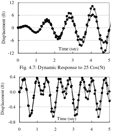
The variation of load f(t) with time in shown in Fig. 4.3. The solutions for u(t) are obtained from Eqs. 4.23 and 4.24 and are plotted in Figs. 4.6~4.8. The main features of these results are
(1) The responses for undamped systems are larger than the damped responses. This is true in general for all three loading cases.
(2) The responses for the second loading case are larger than the other two, because the frequency of the load is equal to the natural frequency of the system. As will be explained later, this is the resonant condition. At resonance, the damped response reaches a maximum amplitude (the steady state amplitude) and oscillates with that amplitude subsequently. This amplitude is 10 ft, which the damped system would
eventually reach if it were allowed to vibrate ‘long enough’. The amplitude of the undamped system, on
the other hand, increases steadily with time and would eventually reach infinity.
Fig. 5.6: Dynamic Response to 25 Cos(2t)
Fig. 4.6: Dynamic Response to 25 Cos(2t)
Fig. 5.7: Dynamic Response to 25 Cos(5t)
Fig. 4.7: Dynamic Response to 25 Cos(5t)
Fig. 5.8: Dynamic Response to 25 Cos(10t)
Dynamic Magnification
In Section 4, it was observed that the maximum dynamic displacements are different from their static counterparts. However, the effect of this magnification (increase or decrease) was more apparent in the harmonic loading case. There, for sinusoidal loads (cosine functions of time) of the same amplitude (25 k) the maximum vibrations varied between 0.5 ft to 12 ft depending on the frequency of the harmonic load.
If the motion is allowed to continue for long (theoretically infinite) durations, the total response converges to the steady state solution given by the particular solution of the equation of motion.
usteady(t) = up(t) = (p0/kd) cos( t ) ………..…(4.19)
[where kd = {(k 2
m)2 + ( c)2}, = tan-1{( c)/ (k 2m)}] Putting the value of kd in Eq. (4.19), the amplitude of steady vibration is found to be
uamplitude = p0/kd = p0/ {(k
Eq. (5.2) gives the ratio of the dynamic and static amplitude of motion as a function of frequency (as well as structural properties like n and ). This ratio is called the steady state dynamic magnification
factor (DMF) for harmonic motion. Putting the frequency ratio / n = r, Eq. (6.2) can be rewritten as
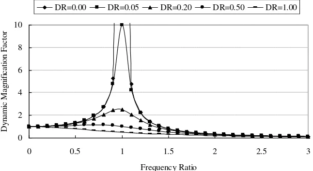
DMF = 1/ {(1 r2)2 + (2 r)2} ..………(5.3)
From which the maximum value of DMF is found to be = (1/2 )/ (1 2), when r = (1 2 2) ……....(5.4)
The variation of the steady state dynamic magnification factor (DMF) with frequency ratio (r = / n) is
shown in Fig. 5.1 for different values of (= DR). The main features of this graph are
1. The curves for the smaller values of show pronounced peaks [ 1/(2 )] at / n 1. This situation is from Section 4 that and vibration amplitude of an undamped system tends steadily to infinity.
3. Since resonance is such a critical condition from structural point of view, it should be avoided in practical structures by making it either very stiff (i.e., r 1) or very flexible (i.e., r 1) with respect to the frequency of the expected harmonic load.
4. The resonant condition mentioned in (1) is not applicable for large values of , because the condition of maxima at r = (1 2 2) is meaningless if r is imaginary; i.e., (1/ 2 =) 0.707. Therefore, another way of avoiding the critical effects of resonance is by increasing the damping of the system.
Fig. 6.1: Steady State Dynamic Magnification Factor
Numerical Solution of SDOF Equation
So far the equation of motion for a SDOF system has been solved analytically for different loading functions. For mathematical convenience, the dynamic loads have been limited to simple functions of time and the initial conditions had been set equal to zero. Even if the assumptions of linear structural
properties and initial ‘at rest’ conditions are satisfied; the practical loading situations can be more complicated and not convenient to solve analytically. Numerical methods must be used in such situations.
The most widely used numerical approach for solving dynamic problems is the Newmark- method. Actually, it is a set of solution methods with different physical interpretations for different values of . The total simulation time is divided into a number of intervals (usually of equal duration t) and the unknown displacement (as well as velocity and acceleration) is solved at each instant of time. The method solves the dynamic equation of motion in the (i + 1)th time step based on the results of the ith step.
The equation of motion for the (i +1)th time step is
m (d2u/dt2)i+1 + c (du/dt)i+1 + k (u)i+1 = f i+1 m ai+1 + c vi+1 + k ui+1 = f i+1 …..………(6.1)
where ‘a’ stands for the acceleration, ‘v’ for velocity and ‘u’ for displacement.
To solve for the displacement or acceleration at the (i + 1)th time step, the following equations are assumed for the velocity and displacement at the (i + 1)th step in terms of the values at the ith step.
vi+1 = vi + {(1 ) ai + ai+1} t ………(6.2)
ui+1 = ui + vi t + {(0.5 ) ai + ai+1} t 2
………(6.3)
By putting the value of vi+1 from Eq. (6.2) and ui+1 from Eq. (6.3) in Eq. (6.1), the only unknown variable
ai+1 can be solved from Eq. (6.1).
In the solution set suggested by the Newmark- method, the Constant Average Acceleration (CAA) method is the most popular because of the stability of its solutions and the simple physical interpretations it provides. This method assumes the acceleration to remain constant during each small time interval t, and this constant is assumed to be the average of the accelerations at the two instants of time ti and ti+1.
The CAA is a special case of Newmark- method where = 0.50 and = 0.25. Thus in the CAA method, the equations for velocity and displacement [Eqs. (6.2) and (6.3)] become
vi+1 = vi + (ai + ai+1) t/2 ………(6.4)
ui+1 = ui + vi t + (ai + ai+1) t 2
/4 ………(6.5)
Inserting these values in Eq. (6.1) and rearranging the coefficients, the following equation is obtained,
(m + c t /2 + k t2/4)ai+1 = fi+1 –kui– (c + k t)vi– (c t/2 + k t 2
/4)ai ….….…..(6.6)
To obtain the acceleration ai+1 at an instant of time ti+1 using Eq. (6.6), the values of ui, vi and ai at the
previous instant ti have to be known (or calculated) before. Once ai+1 is obtained, Eqs. (6.4) and (6.5) can
be used to calculate the velocity vi+1 and displacement ui+1 at time ti+1. All these values can be used to
obtain the results at time ti+2. The method can be used for subsequent time-steps also.
The simulation should start with two initial conditions, like the displacement u0 and velocity v0 at time t0 =
0. The initial acceleration can be obtained from the equation of motion at time t0 = 0 as
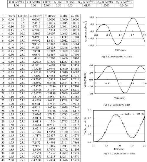
Example 6.1
For the undamped SDOF system described before (m = 1 k-sec2/ft, k = 25 k/ft, c = 0 k-sec/ft), calculate the dynamic response for a Ramped Step Loading with p0 = 25 k and t0 = 0.5 sec.
Results using the CAA Method (for time interval t = 0.05 sec) as well as the exact analytical equation are shown below in tabular form.
Table 6.1: Acceleration, Velocity and Displacement for t = 0.05 sec
Problems on the Dynamic Analysis of SDOF Systems
1. The force vs. displacement relationship of a spring is shown below. If the spring weighs 10 lb, calculate its natural frequency and natural period of vibration. If the damping ratio of the spring is 5%, calculate its damping (c, in lb-sec/in).
2. For the (20 20 20 ) overhead water tank shown below supported by a 25 25 square column, calculate the undamped natural frequency for (i) horizontal vibration (k = 3EI/L3), (ii) vertical vibration (k = EA/L). Assume the total weight of the system to be concentrated in the tank
[Given: Modulus of elasticity of concrete = 400 103 k/ft2, Unit weight of water = 62.5 lb/ft3].
3. The free vibration of an undamped system is shown below. Calculate its
(i) undamped natural period, (ii) undamped natural frequency in Hz and radian/second, (iii) stiffness if its mass is 2 lb-sec2/ft.
4. If a linear viscous damper 1.5 lb-sec/ft is added to the system described in Question 3, calculate its (i) damping ratio, (ii) damped natural period, (ii) free vibration at t = 2 seconds [Initial velocity = 0].
5. The free vibration response of a SDOF system is shown in the figure below. Calculate its
(i) damped natural frequency, (ii) damping ratio, (iii) stiffness and damping if its weight is 10 lb.
6. The free vibration responses of two underdamped systems (A and B) are shown below. (i) Calculate the undamped natural frequency and damping ratio of system B.
(ii) Explain (qualitatively) which one is stiffer and which one is more damped of the two systems.
7. A SDOF system with k = 10 k/ft, m = 1 k-sec2/ft, c = 0 is subjected to a force (in kips) given by (i) p(t) = 50, (ii) p(t) = 100 t, (iii) p(t) = 50 cos(3t).
In each case, calculate the displacement (u) of the system at time t = 0.1 seconds, if the initial displacement and velocity are both zero.
8. Calculate the maximum displacement of the water tank described in Problem 2 when subjected to (i) a sustained wind pressure of 40 psf, (ii) a harmonic wind pressure of 40 cos(2t) psf.
9. An undamped SDOF system suffers resonant vibration when subjected to a harmonic load (i.e., of frequency = n). Of the control measures suggested below, explain which one will minimize the
steady-state vibration amplitude.
(i) Doubling the structural stiffness, (ii) Doubling the structural stiffness and the mass, (iii) Adding a damper to make the structural damping ratio = 10%.
10. For the system defined in Question 7, calculate u(0.1) in each case using the CAA method.
-1.0 -0.5 0.0 0.5 1.0
0.0 0.5 1.0 1.5 2.0
Time (sec)
D
is
pl
ac
em
en
t (
ft
)
Solution of Problems on the Dynamic Analysis of SDOF Systems
1. From the force vs. displacement relationship, spring stiffness k = 200/2.0 = 100 lb/in Weight of the spring is W = 10 lb Mass m = 10/(32.2 12) = 0.0259 lb-sec2/in
Natural frequency, n = (k/m) = (100/0.0259) = 62.16 rad/sec fn= n/2 = 9.89 Hz
Natural period, Tn= 1/fn= 0.101 sec
Damping ratio, = 5% = 0.05
Damping, c = 2 (km) = 2 0.05 (100 0.0259) = 0.161 lb-sec/in
2. Mass of the tank (filled with water), m = 20 20 20 62.5/32.2 = 15528 lb-ft/sec2 Modulus of elasticity E = 400 103 k/ft2 = 400 106 lb/ft2, Length of column L = 30 ft (i) Moment of inertia, I = (25/12)4/12 = 1.570 ft4
Stiffness for horizontal vibration, kh = 3EI/L 3
= 3 400 106 1.570/(30)3 = 69770 lb/ft Natural frequency, nh = (kh/m) = (69770/15528) = 2.120 rad/sec
(ii) Area, A = (25/12)2 = 4.340 ft2
Stiffness for vertical vibration, kv = EA/L = 400 10 6
4.340/30 = 5787 104 lb/ft Natural frequency, nv = (kv/m) = (5787 10
4
/15528) = 61.05 rad/sec
3. (i) The same displacement (2 ft) is reached after 1.0 second intervals. Undamped natural period, Tn = 1.0 sec
(ii) Undamped natural frequency, fn = 1/Tn = 1.0 Hz n = 2 fn = 6.283 radian/second
(iii) Mass, m = 2 lb-sec2/ft. Stiffness, k = m n
2
= 78.96 rad/sec
4. If a linear viscous damper, c = 1.5 lb-sec/ft, (i) damping ratio, (ii) damped natural period, (iii) free vibration at t = 2 seconds [Initial velocity = 0].
(i) Damping ratio, = c/[2 (km)] = 1.5/[2 (78.96 2)] = 0.0597 = 5.97% (ii) Damped natural period, Td = Tn/ (1
2
) = 1.0/ (1 0.05972) = 1.002 sec (iii) Damped natural frequency, d = 2 /Td = 6.272 rad/sec
u(t) = e nt [u0 cos( dt) + {(v0 + nu0)/ d} sin( dt)]
= e 0.0597 6.283 2 [2 cos(6.272 2) + {(0 + 0.0597 6.283 2)/6.272} sin(6.272 2)] = 0.943 ft
5. (i) The figure shows that the peak displacement is repeated in every 1.0 second Damped natural period, Td = 1.0 sec
Damped natural frequency, d = 2 /Td = 6.283 rad/sec
(ii) Damping ratio, = / (1+ 2); where = ln[u(t)/u(t +NTd)]/2 N
Using as reference the displacements at t = 0 (6.0 ft) and t = 2.0 sec (3.0 ft); i.e., for N = 2 = ln[u(0.0)/u(2.0)]/(2 2) = ln[6.0/3.0]/4 = 0.0552 = / (1+ 2) = 0.0551
(iii) Weight, W = 10 lb Mass, m = 10/32.2 = 0.311 lb-sec2/ft Undamped natural frequency, n = d/ (1
2
) = 6.283/ (1 0.05512) = 6.293 rad/sec Stiffness, k = m n2 = 0.311 6.2932 = 12.30 k/ft
and Damping, c = 2 (km) = 2 0.0515 (12.30 0.311) = 0.215 lb-sec/ft
6. (i) System B takes 1.0 second to complete two cycles of vibration. Damped natural period Td for system B = 1.0/2 = 0.50 sec
Damped natural frequency, d = 2 /Td = 12.566 rad/sec
Using as reference the displacements at t = 0 (1.0 ft) and t = 2.0 sec (0.5 ft); i.e., for N = 4 = ln[u(0.0)/u(2.0)]/(2 4) = ln[1.0/0.5]/8 = 0.0276 = / (1+ 2) = 0.0276
(ii) System A completes only two vibrations while (in 2.0 sec) system B completes four vibrations. System B is stiffer.
However, system A decays by the same ratio (i.e., 0.50 or 50%) in two vibrations system B decays in four vibrations.
Mass, m = 15528 lb-ft/sec2, Stiffness for horizontal (i.e., due to wind) vibration, kh = 69770 lb/ft
Natural frequency, nh = 2.120 rad/sec
9. Maximum dynamic response amplitude, umax = p0/(k 2
(iii) Adding a damper to make the structural damping ratio, = 10% = 0.10 umax = p0/ {(k n
2
m)2 + ( nc) 2
} = (p0/k)/(2 ) = 5 (p0/k)
Option (i) is the most effective [since it minimizes umax].
Computer Implementation of Numerical Solution of SDOF Equation
The numerical time-step integration method of solving the SDOF dynamic equation of motion using the Newmark- method or its special case CAA (Constant Average Acceleration) method can be used for any dynamic system with satisfactory agreement with analytical solutions. Numerical solution is the only option for problems that cannot be solved analytically. They are particularly useful for computer implementation, and are used in the computer solution of various problems of structural dynamics. These are implemented in standard softwares for solving structural dynamics problems.
A computer program written in FORTRAN77 for the Newmark- method is listed below for a general linear system and dynamic loading. Although the forcing function is defined here (as the Ramped Step Function mentioned before) the algorithm can be used in any version of FORTRAN to solve dynamic SDOF problems, with slight modification for the forcing function. Also, the resulting acceleration, velocity and displacement are printed out only once in every twenty steps solved numerically. This can also be modified easily depending on the required output. The program listing is shown below.
OPEN(1,FILE='SDOF.IN',STATUS='OLD') OPEN(2,FILE='OUT',STATUS='NEW')
READ(1,*)RM0,RK0,DRATIO READ(1,*)DT,NSTEP
C0=2.*DRATIO*SQRT(RK0*RM0) TIME=0.
DIS0=0. VEL0=0. FRC=0.
ACC0=(FRC RK0*DIS0 C0*VEL0)/RM0 WRITE(2,4)TIME,ACC0,VEL0,DIS0 RKEFF=RK0
CEFF=C0+RK0*DT
RMEFF=C0*DT/2.+RK0*DT**2/4. DO 10 I=1,NSTEP
TIME=DT*I FRC=25.
IF(TIME.LE.0.5)FRC=50.*TIME
ACC=(FRC-RKEFF*DIS0 CEFF*VEL0-RMEFF*ACC0)/(RM0+RMEFF) VEL=VEL0+(ACC0+ACC)*DT/2.
DIS=DIS0+VEL0*DT+(ACC0+ACC)*DT**2/4. IF(I/20.EQ.I/20.)WRITE(2,4)TIME,ACC,VEL,DIS DIS0=DIS
VEL0=VEL ACC0=ACC 10 CONTINUE
Example 7.1
For the SDOF system described before (m = 1 k-sec2/ft, k = 25 k/ft) with damping ratio = 0 (c = 0 k-sec/ft), calculate the dynamic displacements for a Ramped Step Loading with p0 = 25 k and t0 = 0.5 sec.
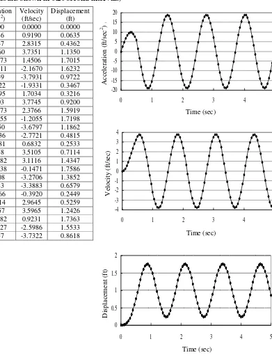
The output file for the FORTRAN77 program listed in the previous section is shown below in tabular form (in Table 7.1). The numerical integrations are carried out for time intervals of t = 0.01 sec and results are printed in every 0.20 second up to 5.0 seconds.
Table 7.1: Acceleration, Velocity and Displacement for t = 0.01 sec(Results shown in 0.20 second intervals)
Time
Fig. 8.1: Acceleration, Velocity & Displacement vs. Time 0
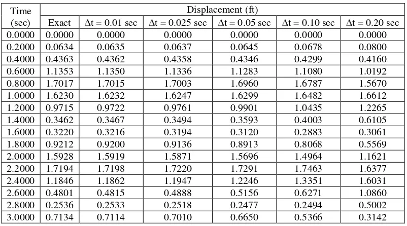
The numerical results (i.e., displacements only) obtained for t = 0.01 are presented in Table 7.2 along with exact analytical results and results for t = 0.025 and 0.05 sec. In the table, it is convenient to notice the deterioration of accuracy with increasing t, although those results are also very accurate and the deterioration of accuracy cannot be detected in Fig. 7.2, where they are also plotted.
Numerical predictions are worse for larger t but the CAA guarantees convergence for any value of t, even if the results are not very accurate. Table 7.2 also shows the results for t = 0.10 and 0.20 sec. These results are clearly unsatisfactory compared to the corresponding exact results, but overall there is only a shift in the dynamic responses and there if no tendency to diverge towards infinity.
Table 7.2: Exact Displacement and Displacement for t = 0.01, 0.025, 0.05, 0.10, 0.20 sec
Time (sec)
Displacement (ft)
Exact t = 0.01 sec t = 0.025 sec t = 0.05 sec t = 0.10 sec t = 0.20 sec
0.0000 0.0000 0.0000 0.0000 0.0000 0.0000 0.0000
0.2000 0.0634 0.0635 0.0637 0.0645 0.0678 0.0800
0.4000 0.4363 0.4362 0.4358 0.4346 0.4299 0.4160
0.6000 1.1353 1.1350 1.1336 1.1283 1.1080 1.0192
0.8000 1.7017 1.7015 1.7003 1.6960 1.6787 1.5670
1.0000 1.6230 1.6232 1.6247 1.6299 1.6482 1.6612
1.2000 0.9715 0.9722 0.9761 0.9901 1.0435 1.2265
1.4000 0.3462 0.3467 0.3494 0.3593 0.4003 0.6105
1.6000 0.3220 0.3216 0.3194 0.3120 0.2883 0.3061
1.8000 0.9212 0.9200 0.9136 0.8913 0.8068 0.5569
2.0000 1.5928 1.5919 1.5871 1.5696 1.4964 1.1621
2.2000 1.7194 1.7198 1.7220 1.7291 1.7463 1.6377
2.4000 1.1846 1.1862 1.1947 1.2246 1.3351 1.6031
2.6000 0.4801 0.4815 0.4888 0.5156 0.6271 1.0860
2.8000 0.2536 0.2533 0.2518 0.2477 0.2494 0.5002
3.0000 0.7134 0.7114 0.7010 0.6650 0.5366 0.3142
The accuracy of the results depends on the choice of t with respect to the natural period of the system or the period of the forcing function itself. For example, whereas t = 0.1 and 0.2 sec do not give accurate results for the given system (with natural frequency = 5.0 rad/sec, natural period = 1.257 seconds) it gives much more accurate predictions for ‘System2’ where m = 1 k-sec2/ft and k = 4 k/ft (i.e., natural frequency = 2 rad/sec, natural period = 3.142 seconds). The results are shown in Table 7.3.
Table 7.3: Exact Displacement and Displacement for t = 0.1 and 0.2 sec for System2
Time (sec) [Exact] [ t = 0.1 sec] [ t = 0.2 sec]
0.0000 0.0000 0.0000 0.0000
0.2000 0.0661 0.0738 0.0962
0.4000 0.5165 0.5281 0.5621
0.6000 1.6664 1.6714 1.6628
0.8000 3.5317 3.5205 3.4211
1.0000 5.8261 5.7978 5.6146
1.2000 8.1874 8.1459 7.9059
1.4000 10.2429 10.1967 9.9424 1.6000 11.6679 11.6284 11.4109 1.8000 12.2376 12.2166 12.0853 2.0000 11.8620 11.8689 11.8621 2.2000 10.6004 10.6399 10.7754
2.4000 8.6519 8.7224 8.9926
2.6000 6.3242 6.4170 6.7877
2.8000 3.9848 4.0855 4.5002
Fig. 8.3: Displacement vs. Time for 'large' time steps 0 Fig. 8.2: Displacement vs. Time for different time steps
0
Exact time step=0.01 sec time step=0.025 sec time step=0.05 sec
Fig. 8.4: Displacement vs. Time for System2
Introduction to Multi-Degree-of-Freedom (MDOF) System
The lectures so far had dealt with Single-Degree-of-Freedom (SDOF) systems, i.e., systems with only one displacement. Although important concepts like free vibration, natural frequency, forced vibration, dynamic magnification and resonance were explained, the conclusions based on such a simplified model have limitations while applying to real structures. Real systems can be modeled as SDOF systems only if it is possible to express the physical properties of the system by a single motion. However, in most cases the SDOF system is only a simplification of real systems modeled by assuming simplified deflected shapes that satisfy the essential boundary conditions.
Real structural systems often consist of an infinite number of independent displacements/rotations and need to be modeled by several degrees of freedom for an accurate representation of their structural response. Therefore, real structural systems are called Multi-Degree-of-Freedom (MDOF) systems in contrast to the SDOF systems discussed before.
A commonly used dynamic model of a 1-storied building is as shown in Fig. 8.1(b), represented by the story sidesway only. Since weight carried by the building is mainly concentrated at the slab and beams while the columns provide the resistance to lateral deformations, the SDOF model assumes a spring and a dashpot for the columns and a mass for the slabs. However the SDOF model may not be an adequate model for real building structures, which calls for modeling as MDOF systems. The infinite number of deflections and rotations of the 1-storied frame shown in Fig. 8.1(a) (subjected to the vertical and horizontal loads as shown) can also be represented by the joint displacements and rotations. A detailed formulation of the 1-storied building frame would require at least three degrees of freedom per joint; i.e., twelve degrees of freedom overall for the four joints (reduced to six after applying boundary conditions). The models become even more complicated for larger structures.
(a) (b)
Fig. 8.1: One-storied building frame (a) with infinite degrees of freedom, (b) modeled as a SDOF system
Some of the comparative features of the SDOF and MDOF systems are
1. Several basic concepts used for the analysis of SDOF systems like free and forced vibration, dynamic magnification can also be used for MDOF systems.
2. However, some differences between the analyses of SDOF and MDOF systems are mainly due to the more elaborate nature of the MDOF systems. For example, the basic SDOF concepts are valid for each degree of freedom in a MDOF system. Therefore, the MDOF system has several natural frequencies, modes of vibration, damping ratios, modal masses.
Formulation of the 2-DOF Equations for Lumped Systems
The simplest extension of the SDOF system is a two-degrees-of-freedom (2-DOF) system, i.e., a system with two unknown displacements for two masses. The two masses may be connected to each other by several spring-dashpot systems, which will lead to two differential equations of motion, the solution of which gives the displacements and internal forces in the system.
Fig. 8.2: Dynamic 2-DOF system and free body diagrams of m1 and m2
Fig. 8.2 shows a 2-DOF dynamic system and the free body diagrams of the two masses m1 and m2. In the
figure, ‘u’ stands for displacement (i.e., u1 and u2) while ‘v’ stands for velocity (v1 and v2). Denoting
accelerations by a1 and a2, the differential equations of motion can be applied by applying Newton’s 2 nd (8.1) and (8.2), the following equations are obtained
m1 d
Eqs. (8.3) and (8.4) can be arranged in matrix form as m1 0 d
Eqs. (8.5) represent in matrix form the set of equations [i.e. (8.3) and (8.4)] to evaluate the displacements u1(t) and u2(t). In this set, the matrix consisting of the masses (m1 and m2) is called the mass matrix, the
one consisting of the dampings (c1 and c2) is called the damping matrix and the one consisting of the
stiffnesses (k1 and k2) is called the stiffness matrix of this particular system. These matrices are different
for various 2-DOF systems, so that Eq. (8.5) cannot be taken as a general form of governing equations of motion for any 2-DOF system.
For a MDOF system, the mass, damping and stiffness matrices can be generalized by their coefficients, so that Eq. (8.5) can be written in the general form of the dynamic equations of motion,
Eigenvalue Problem and Calculation of Natural Frequencies of a MDOF System
In the previous section, the general equations of motion of a general MDOF system was mentioned to be
M d2u/dt2+ C du/dt+ K u = f(t) ……….….(8.6)
The free vibration condition for the dynamic motion of MDOF system is obtained by setting f(t) = 0; i.e.,
M d2u/dt2+ C du/dt+ K u = 0 ……….….(9.1)
In order to obtain the natural frequency of the undamped system, if C is also set equal to zero, the equations of motion reduce to
M d2u/dt2+ K u = 0 ……….….(9.2)
If the displacement vector can be chosen as the summation of a number (equal to the DOF) of variable
separable vectors u(t) = qr(t) r ………..(9.3)
where qr(t) is a time-dependent scalar and r is a space-dependent vector.
With q(t) = Ar e i nrt
, or qr(t) = C1r cos ( nrt) + C2r sin ( nrt) .………...………..(9.4)
Eq. (9.2) can be written as [ nr 2
M + K] qr(t) r= 0 [K nr
2
M] r = 0 ……….….(9.5)
Since the vector u is not zero, Eq. (9.5) turns into the following eigenvalue problem
K nr 2
M = 0 ……….….(9.6)
i.e., the determinant of the matrix (K nr2M) is zero.
Eq. (9.6) is satisfied for different values of the ‘natural frequency’ nr, which implies that there can be
several natural frequencies of a MDOF system. In fact, the number of natural frequencies of the system is equal to the degrees of freedom of the system, i.e., size of the displacement vector. However, consideration of only the first few can adequately model the structural behavior of a dynamic system.
There are several ways to solve the eigenvalue problem of Eq. (9.6), the suitability of which depends on the size of the matrices and the number of eigenvalues required to represent the system accurately.
For each value of nr, the vector ris called a modal vector for the r
th
mode of vibration. Once a natural frequency is known, Eq. (9.5) can be solved for the corresponding vector r to within a multiplicative
constant. The eigenvalue problem does not fix the absolute amplitude of the vectors r, only the shape of
the vector is given by the relative values of the displacements.
Thus the vector r (i.e., the eigenvectors, also called the natural mode of vibration, normal mode, characteristic vector, etc.) physically represents the modal shape of the system corresponding to the natural frequency. The relative values of the displacements in the vector r indicate the shape that the structure would assume while undergoing free vibration at the relevant natural frequency.
The undamped natural frequencies and modal shapes calculated from the above procedure usually prove to be adequate in the subsequent dynamic analyses, since the damped natural frequencies are often quite similar to the damped natural frequencies for typical (undamped) systems, as mentioned in the discussion on SDOF systems.
However, the damped natural frequencies and modal shapes can also be calculated by the methods mentioned before. For that, qr(t) = Ar e
i nrt
will lead to the following equation
[K +i nrC nr 2
M] r = 0 K +i nr C nr 2
M = 0 ………..….….(9.7)
Example 9.1
Calculate the natural frequencies and determine the natural modes of vibration of the 2-storied building system shown in Figs. 8.1 and 8.2, whose governing equations of motion are given by Eq. (8.5). Assume, k1 = k2 = 25 k/ft, m1 = m2 = 1 k-sec
2
/ft, c1 = c2 = 0 (i.e., the same stiffnesses and masses as used for the
SDOF system before are used here for an undamped 2-DOF system).
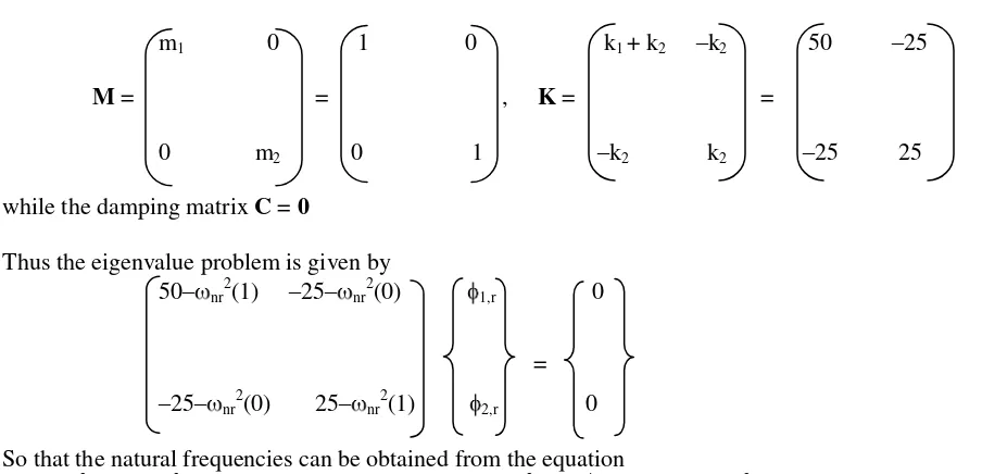
Solution
Thus the eigenvalue problem is given by 50– nr
So that the natural frequencies can be obtained from the equation (50– nr
The two values of the natural frequency indicate the first and second natural frequency of the system.
n1 = 3.09 and n2 = 8.09 rad/sec for this system.
[Recall that the natural frequency n was equal to 5 rad/sec (i.e., fn = 0.796 cycle/sec) for the SDOF
system in Example 2.1, which is greater than n1 but less than n2]
Once the natural frequencies are known, modal shapes can be determined from the eigenvalue equation. For the first natural frequency, the eigenvalue equations are
40.45 –25 1,1 0
=
–25 15.45 2,1 0
from both these equation, 1.618 1,1– 2,1 = 0 1,1 : 2,1 = 1: 1.618
For the second natural frequency, the equations are
–15.45 –25 1,2 0
=
–25 –40.45 2,2 0
from both these equations, – 1,2– 1.618 2,2 = 0 1,2 : 2,2 = 1: –0.618
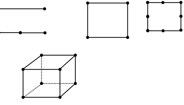
Thus, the first two modal shapes are as shown in Fig. 9.1.
First Mode Second Mode Fig. 9.1: Modal Shapes of the system
1.0 1.618
1.0 0.618
Modal Analysis of MDOF Systems
Calculation of the natural frequencies and the corresponding natural modes of vibration are important in developing a general method of dynamic analysis called the Modal Analysis. This method decomposes the dynamic system into different SDOF systems after solving the eigenvalue problem for natural frequencies and natural modes and considers the individual modes separately to obtain the total solution.
The Modal Analysis uses a very important characteristic of the modal vectors, i.e., the orthogonality conditions. The derivation of the orthogonality conditions is avoided here, but they are available in any standard text on Structural Dynamics. If ni and nj are the i
th
and jth natural frequencies of an undamped system and i and j are the ith and jth modes of vibration, then if j i, the mass and stiffness matrices
where the superscripts T indicate the transpose of the matrices. If j = i, the ratio of the products i T
natural frequency of the system; i.e.,
ni
Choosing the displacement vector as the summation of a number (equal to the DOF) of variable separable vectors [using Eq. (9.3)]
Using the orthogonality equations ( i T
mode of the system. Eq. (10.6) is an uncoupled differential equation that can be solved to get qi(t) as a function of time.
Since i is already known by solving the eigenvalue problem, qi(t) can be inserted in Eq. (9.3) and
summing up similar components gives u(t). Therefore, the main advantage of the orthogonality conditions is to uncouple the equations of motion so that they can be solved as separate SDOF systems.
For a damped system, the damping matrix C can also be formed to satisfy orthogonality condition; i.e.,
jT C i = 0 ………..(10.7)
This can be possible if the matrix C is proportional to the mass matrix M or the stiffness matrix K, or more rationally a combination of the two; i.e.,
C = a0M + a1K ………..(10.8)
Thus formulated, the equation of motion for the ith mode can be written as ( i
Example 10.1
For the 2-storied building system described in Example 9.1, calculate the dynamic displacement vector if step loads of 25 kips are applied at both stories when the system is at rest; i.e., f1(t) = f2(t) = 25 kips.
Solution
The mass and stiffness matrices of the system are given by
m1 0 1 0 k1 + k2 –k2 50 –25
M = = , K = =
0 m2 0 1 –k2 k2 –25 25
while the damping matrix C = 0
From Example 9.1, the natural frequencies of the system are found to be
n1 = 3.09 rad/sec, and n2 = 8.09 rad/sec, while the modal vectors are given by
1 1
1= and 2 =
1.618 –0.618
The modal masses are, M1 = 1 T
M 1 = 3.618 k-sec
2
/ft, M2 = 2 T
M 2 = 1.382 k-sec
2
/ft
The modal stiffnesses are, K1 = 1 T
K 1 = 34.55 k/ft, K2 = 2 T
K 2 = 90.45 k/ft
The modal loads are, f1(t) = 1 T
f = 65.45 k, f2(t) = 2 T
f = 9.55 k
The uncoupled modal equations of motion are 3.618 d2q1/dt
2
+ 34.55q1 = 65.45
1.382 d2q2/dt 2
+ 90.45q2 = 9.55
The solution of these equations starting ‘at rest’ is
q1(t) = (65.45/34.55) [1– cos (3.09t)] = 1.894 [1– cos (3.09t)]
and q2(t) = (9.55/90.45) [1– cos (8.09t)] = 0.1056 [1– cos (8.09t)]
u(t) = qi(t) i = q1(t) 1 + q2(t) 2
1 1
u(t)= 1.894 [1– cos (3.09t)] + 0.1056 [1– cos (8.09t)]
1.618 –0.618
u1(t) = 1.894 [1– cos (3.09t)] + 0.1056 [1– cos (8.09t)]
u2(t) = 3.065 [1– cos (3.09t)] – 0.065 [1– cos (8.09t)]
The displacements are plotted with time in Fig. 10.1 and 10.2. Fig. 10.1 shows the contribution of the two modes to the total displacements, which are shown in Fig. 10.2. The figures indicate that u2 is larger in
In Example 10.1, the modal masses were calculated to be M1 = 3.618 k-sec 2
/ft, M2 = 1.382 k-sec 2
/ft, and in Example 9.1, the natural frequencies of the system were found to be
n1 = 3.09 rad/sec, and n2 = 8.09 rad/sec
Using Eq. (10.10), the modal damping ratios are
1 = C1/(2M1 n1) = 0.691/(2 3.618 3.09) = 0.0309 2 = C2/(2M2 n2) = 1.809/(2 1.382 8.09) = 0.0809
1 is lower while 2 is greater than 0.05. Particularly the damping ratio of the second mode is much higher,
which helps to suppress it even further.
Fig. 12.1: Contribution of various Modes
u1, Mode1 u2, Mode1 u1, Mode2 u2, Mode2
Numerical Solution of MDOF Equations
The equations of motion for a MDOF system have been solved analytically using the Modal Analysis. Although Modal Analysis is helpful in formulating and understanding some basic concepts of dynamic analysis, it has several limitations of convenience and applicability. In fact, it has even more limitations than the analytical methods used to solve SDOF systems.
In addition to the considerable mathematical effort needed to solve eigenvalue problems and uncouple the simultaneous equations (i.e., make the system matrices diagonal), its formulation requires several assumptions. For example, the method is valid for linear systems only. The orthogonality condition that makes the Modal Analysis convenient, is not guaranteed to be valid for the damping matrix. The practical loading situations can be more complicated and not convenient to solve analytically. Numerical methods must be used in such situations.
As mentioned for SDOF systems, the most widely used numerical approach for solving dynamic problems is the Newmark- method. The method solves the dynamic equation of motion in the (i+1)th time step based on the results of the ith step.
The dynamic equations of motion for the (i+1)th time step is
M ai+1+ C vi+1+ K ui+1 = f i+1 ..………(11.1)
where the bold small letter ‘a’ stands for the acceleration vector, ‘v’ for velocity vector and ‘u’ for
displacement vector. In the Constant Average Acceleration (CAA) method (a special case of Newmark-
method where = 0.50 and = 0.25), the velocity and displacement vectors are given by
vi+1 = vi + (ai + ai+1) t/2 ………(11.2)
ui+1 = ui + vi t + (ai + ai+1) t2/4 ………(11.3)
Inserting these values in Eq. (13.1) and rearranging the coefficients, the following equation is obtained, (M + C t /2 + K t2/4)ai+1= fi+1–Kui– (C + K t)vi– (C t/2 + K t2/4)ai …………...…..(11.4)
Therefore, if the forcing function fi+1 is known, the only unknown in Eq. (11.4) is the acceleration vector
ai+1, which can be obtained by matrix inversion (by Gauss Elimination or some other method). Once ai+1is obtained, Eqs. (11.2) and (11.3) can be used to calculate the velocity vector vi+1and the displacement vector ui+1at time ti+1. These values are used to obtain the results at time ti+2 and subsequent time-steps.
The simulation needs two initial conditions, e.g., the displacement vector u0and velocity vector v0 at time t0 = 0. Then the initial acceleration vector can be obtained as
a0= M-1(f0–Cv0–Ku0) ………(11.5)
Again, any standard method of matrix inversion can be used to solve Eq. (11.5).
Among other methods of numerical solution of the MDOF equations of motion, the Linear Acceleration
method and Central Difference method are quite popular. The Linear Acceleration Method is a special case of the Newmark- method with = 0.50 and = 1/6. Instead of assuming constant average acceleration between two time intervals, it assumes the acceleration to vary linearly in between two intervals. Unlike the CAA method, the Linear Acceleration method is not unconditionally stable. However, the time increment needed for its stability is much greater than the interval needed for accurate results, therefore stability is usually not a problem for this method.
Computer Implementation of Numerical Solution of MDOF Equations
The numerical time-step integration method of solving the MDOF dynamic equation of motion has been described in the previous section. Just as the computer implementation in SDOF system, the Constant Average Acceleration (CAA) method can be used for any dynamic system with satisfactory agreement with analytical solutions.
A computer program written in FORTRAN77 for the CAA method is listed below for a general linear system and dynamic loading. The forcing function is defined here as the Step Function, but the algorithm can be used in any version of FORTRAN to solve dynamic MDOF problems with slight modification for the forcing function, which can be used as input also. Besides, the stiffness, damping and mass matrices are input for the discrete systems, but in practice they can be assembled from structural properties. The resulting displacements are printed only once in every ten steps solved numerically. This can also be modified easily depending on the required output. The program listing is shown below.
PROGRAM MDOF
DIMENSION DIS(100),VEL(100),ACC(100),DISV(100),VELV(100) DIMENSION DIS0(100),VEL0(100),ACC0(100),FORCE(100) DIMENSION SK(100,100),SC(100,100),SM(100,100)
COMMON/SOLVER/SMEFF(100,100),PEFF(100),NDF OPEN(1,FILE='MDOF.IN',STATUS='OLD')
OPEN(2,FILE='MDOF.OUT',STATUS='NEW') PI=4.*ATAN(1.)
READ(1,*)NDF
READ(1,*)((SK(I,J),J=1,NDF),I=1,NDF) READ(1,*)((SC(I,J),J=1,NDF),I=1,NDF) READ(1,*)((SM(I,J),J=1,NDF),I=1,NDF)
C*******TIME-STEP INTEGRATION USING CAA METHOD****************
READ(1,*)DSTEP,NSTEP
A1=DSTEP/2. A2=DSTEP**2/4.
READ(1,*)(DIS0(I),VEL0(I),FORCE(I),I=1,NDF)
C*******INITIAL ACCELERATION********************************** DO 16 I=1,NDF
DO 16 J=1,NDF SMEFF(I,J)=SM(I,J) 16 CONTINUE
DO 18 I=1,NDF PEFF(I)=FORCE(I) DO 18 J=1,NDF
PEFF(I)=PEFF(I)–SC(I,J)*VEL0(J)–SK(I,J)*DIS0(J) 18 CONTINUE
CALL GAUSS DO 19 I=1,NDF 19 ACC0(I)=PEFF(I)
WRITE(2,6)TIME,(DIS0(I),I=1,NDF) 6 FORMAT(10(1X,F8.4))
VELV(I)=VEL0(I)+ACC0(I)*A1
27 DISV(I)=DIS0(I)+VEL0(I)*DSTEP+ACC0(I)*A2
DO 28 I=1,NDF PEFF(I)=FORCE(I) DO 28 J=1,NDF
PEFF(I)=PEFF(I)–SC(I,J)*VELV(J)–SK(I,J)*DISV(J) 28 CONTINUE
DO 15 I=1,NDF DO 15 J=1,NDF
SMEFF(I,J)=SM(I,J)+SC(I,J)*A1+SK(I,J)*A2 15 CONTINUE
CALL GAUSS DO 29 I=1,NDF ACC(I)=PEFF(I)
VEL(I)=VEL0(I)+(ACC0(I)+ACC(I))*A1
DIS(I)=DIS0(I)+VEL0(I)*DSTEP+(ACC0(I)+ACC(I))*A2 DIS0(I)=DIS(I)
VEL0(I)=VEL(I) 29 ACC0(I)=ACC(I)
C********DISPLACEMENTS**************************************** IF(IT/10.EQ.IT/10.)WRITE(2,6)TIME,(DIS(I),I=1,NDF)
26 CONTINUE 20 END
C**************************************************************** C*******GAUSS ELIMINATION*************************************
SUBROUTINE GAUSS
COMMON/SOLVER/AG(100,100),BG(100),N N1=N–1
DO 10 I=1,N1 I1=I+1 CG=1./AG(I,I) DO 11 KS=I1,N DG=AG(KS,I)*CG DO 12 J=I1,N
12 AG(KS,J)=AG(KS,J)–DG*AG(I,J) 11 BG(KS)=BG(KS)–DG*BG(I) 10 CONTINUE
BG(N)=BG(N)/AG(N,N) DO 13 II=1,N1
I=N–II I1=I+1 SUM=0. DO 14 J=I1,N
14 SUM=SUM+AG(I,J)*BG(J) 13 BG(I)=(BG(I)–SUM)/AG(I,I)
Example 11.1
For the 2-DOF system described before (m1 = m2 = 1 k-sec 2
/ft, k1 = k2 = 25 k/ft) with damping ratio = 0.0
or similar damping as the SDOF system with 5% damping (c1 = c2 = 0.5 k-sec/ft), calculate the dynamic
displacements for a Step Loading with f1 = f2 = 25 k.
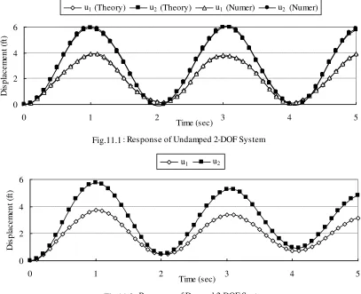
The results from the FORTRAN77 program listed in the previous section are plotted in Fig. 11.1 and Fig. 11.2. The numerical integrations are carried out for time intervals of t = 0.01 sec and results are printed in every 0.10 second up to 5.0 seconds.
Fig. 11.1 shows that the results from the numerical method can hardly be distinguished from the theoretical results obtained from Modal Analysis. The maximum values of the displacements (u1 and u2)
are 3.92 ft and 6.00 ft respectively. Since the static displacements in this case are u1 = 2 ft, u2 = 3 ft, the
dynamic magnifications are nearly 2.
Example 11.2
For a 4-DOF system with structural properties similar to the 2-DOF system described before (m1 = m2 =
m3 = m4 = 1 k-sec 2
/ft, k1 = k2 = k3 = k4 = 25 k/ft) with similar damping as the SDOF system with 5%
damping (c1 = c2 = c3 = c4 = 0.5 k-sec/ft), calculate the dynamic displacements for a Step Loading with f1
= f2 = f3 = f4 = 25 k.
This problem is difficult to solve analytically because it involves solution of a 4 4 matrix. However, the numerical method is used here easily using the computer program listed before. The resulting dynamic displacements are shown in Fig. 11.3. The maximum values of u1, u2, u3 and u4 are 7.56, 13.55, 17.58 and
19.5 ft respectively, reached at the first peak at nearly 1.8 seconds. This shows that the fundamental time period of this system is about 3.6 seconds and since the static solutions of u1, u2, u3 and u4 are 4, 7, 9 and
10 ft respectively, the dynamic magnifications are nearly 2 again for all the displacements.
Fig. 14.3: Response of Damped 4-DOF System 0
5 10 15 20
0 1 2 3 4 5
Time (sec)
D
is
p
la
c
e
m
e
n
t
(f
t)
u1 u2 u3 u4
Fig.11.3
Problems on the Dynamic Analysis of MDOF Systems
1. A small structure of stiffness 1 k/ft, natural frequency 1 rad/sec and damping 1 k-sec/ft is mounted on a larger undamped structure of stiffness 10 k/ft but the same natural frequency. Determine the
(i) natural frequencies, (ii) natural modes of vibration, (iii) modal damping ratios of the system.
2. For a (20 20 ) floor system weighing 200 psf (including all dead and live loads) supported by four (10 10 ) square columns (each 12 high) and a rigid massless footing, calculate the undamped natural period for horizontal vibration.
Consider k for each column = 12EI/L3 and kf for footing equal to (i) 2 10 6
lb/in, (ii) 2 104 lb/in. Assume the total weight of the system to be concentrated at the floor
[Given: Modulus of elasticity of concrete = 3 106 psi].
3. A 2-DOF system is composed of two underdamped systems (A and B), whose free vibration responses are shown below. If each system weighs 100 lb, calculate the
(i) undamped natural frequency and damping ratio of system A and B, (ii) first natural frequency and damping ratio of the 2-DOF system formed.
4. A lumped-mass 3-DOF dynamic system has the following properties k1 = k2 = k3 = 50 k/ft, c1 = c2 = c3 = 1 k-sec/ft, m1 = m2 = m3 = 2 k-sec
2
/ft. (i) Form the stiffness, damping and mass matrices of the system.
(ii) Calculate the 1st natural frequency and damping ratio of the system, if the 1st modal vector for the system is given by 1 = {0.445, 0.802, 1.000}T.
5. The undamped 2-DOF system described in the class is subjected to harmonic load vectors of (i) f(t)= {0, 50 cos(3t)}T, (ii) f(t)= {0, 50 cos(8t)}T.
In both cases, calculate the displacement vector u(t) of the system at time t = 0.1 seconds, if the system is initially at rest.
6. Calculate the maximum floor displacement of the system described in Question 2 when subjected to a horizontal step load of 10 kips at the floor level.
7. For the system defined in Question 5, calculate u(0.1) in each case using the CAA method.
-1.0 -0.5 0.0 0.5 1.0
0.0 0.5 1.0 1.5 2.0
Time (sec)
D
is
pl
ac
em
en
t (
ft
)
Solution of Problems on the Dynamic Analysis of MDOF Systems
The eigenvalue problem (11 10 n
2
The eigenvalue problem (613.02 3.11 n
2
) (490.42 3.11 n
2
) ( 490.42)2 = 0
n = 4.30, 18.35 rad/sec n1= 4.30 rad/sec
The natural frequencies are n1 = 3.09 rad/sec, n2 = 8.09 rad/sec The uncoupled modal equations of motion are
Dynamic Equations of Motion for Continuous Systems
The basic concepts of Structural Dynamics discussed so far dealt with discrete dynamic systems; i.e., with Single-Degree-of-Freedom (SDOF) systems and Multi-Degree-of-Freedom (MDOF) systems. The fundamental equations of motion were derived using Newton’s 2nd law of motion. While this is useful for dealing with most problems involving point masses and forces, there are certain problems where such formulations are not convenient.
Method of Virtual Work
Another way of representing Newton’s equations of static and dynamic equilibrium is by energy methods, which is based on the law of conservation of energy. According to the principle of virtual work, if a system in equilibrium is subjected to virtual displacements u, the virtual work done by the external forces ( WE) is equal to the virtual work done by the internal forces ( WI)
WI = WE …...………(12.1)
where the symbol is used to indicate ‘virtual’. This term is used to indicate hypothetical increments of displacements and works that are assumed to happen in order to formulate the problem.
Energy Formulation for Discrete SDOF System:
If a virtual displacement u is applied on a SDOF system with a single mass m, a damping c and stiffness k undergoing displacement u(t) due to external load f(t),
the virtual internal work, WE = f(t) u ………(12.2)
and virtual external work, WI = m d2u/dt2 u + c du/dt u + k u u ………(12.3)
Combining m d2u/dt2 u + c du/dt u + k u u = f(t) u m d2u/dt2 + c du/dt+ k u= f(t) …...…(12.4)
which is the same as Eq. (2.5), derived earlier from Newton’s 2nd
law of motion.
So, the method of virtual work leads to the same conclusion as the equilibrium formulation. This method is not very convenient here, but its advantage is more apparent in the formulation for continuous systems.
Energy Formulation for Continuous SDOF Systems:
Most of the practical dynamic problems involve continuous structural systems. Unlike discrete MDOF systems, these continuous systems can only be defined properly by an infinite number of displacements; i.e., infinite degrees of freedom.
However several continuous systems are modeled as SDOF systems by assuming all the displacements as proportional to a single displacement (related by an appropriate deflected shape as a function of space). The governing equations from such assumed deflected shapes are similar to SDOF equations with the
‘equivalent’ mass m*, damping c*, stiffness k* and load f*(t) being the essential parameters instead of the respective discrete values m, c, k and f(t).
Therefore, once the appropriate defected shapes are assumed and the ‘equivalent’ parameters calculated,