A Complete Introduction on Bachelor of Science Level

(1)

Dr Wolfgang Schärtl

Basic Physical Chemistry

(2)

Dr Wolfgang Schärtl

Basic Physical Chemistry

(3)

Download free eBooks at bookboon.com

3

Basic Physical Chemistry: A Complete Introduction on Bachelor of Science Level

1

st

edition

bookboon.com

(4)

Contents

Biography of Dr. Wolfgang Schaertl 6

Prologue 7

1 Mathematical Basics 9

1.1 Differentials and simple differential equations 9

1.2 Logarithms and trigonometric functions 11

1.3 Linearization of mathematical functions, and Taylor series expansion 12 1.4 Treating experimental data – SI-system and error calculation 14

2 Thermodynamics 17

2.1 Definitions 17

2.2 Gas equations 19

2.3 The fundamental laws of thermodynamics 32

2.4 Heat capacities 47

www.sylvania.com

We do not reinvent

the wheel we reinvent

light.

Fascinating lighting offers an infinite spectrum of possibilities: Innovative technologies and new markets provide both opportunities and challenges. An environment in which your expertise is in high demand. Enjoy the supportive working atmosphere within our global group and benefit from international career paths. Implement sustainable ideas in close cooperation with other specialists and contribute to influencing our future. Come and join us in reinventing light every day.

(5)

Click on the ad to read more Basic Physical Chemistry

5

Contents

2.5 Phase equilibrium 50

2.6 The chemical equilibrium 81

2.7 Reaction energy 85

3 Kinetics 87

3.1 Elementary reactions (one single reaction step, molecularity = order) 89 3.2 The kinetics of more complex multistep chemical reactions 95

3.3 Activation energy 98

4 Electrochemistry 101

4.1 Electric Conductivity 101

4.2 The electrochemical potential and electrochemical cells 120

5 Introduction to Quantum Chemistry and Spectroscopy 133

5.1 Models of the atom 133

5.2 The wave character of matter, or the wave-particle-dualism 138 5.3 Mathematical solutions of some simple problems in quantum mechanics:

particle in a box, harmonic oscillator, rotator and the hydrogen atom 145 5.4 A brief introduction to optical spectroscopy 154

Subject index 164

EADSunites a leading aircraft manufacturer, the world’s largest helicopter supplier, a global leader in space programmes and a worldwide leader in global security solutions and systems to form Europe’s largest defence and aerospace group. More than 140,000 people work at Airbus, Astrium, Cassidian and Eurocopter,

in 90 locations globally, to deliver some of the industry’s most exciting projects.

An EADS internship offers the chance to use your theoretical knowledge and apply it first-hand to real situations and assignments during your studies. Given a high level of responsibility, plenty of

learning and development opportunities, and all the support you need, you will tackle interesting challenges on state-of-the-art products.

We welcome more than 5,000 interns every year across disciplines ranging from engineering, IT, procurement and finance, to strategy, customer support, marketing and sales. Positions are available in France, Germany, Spain and the UK.

To find out more and apply, visit www.jobs.eads.com. You can also find out more on our EADS Careers Facebookpage.

(6)

Biography of Dr. Wolfgang Schaertl

Wolfgang Schaertl was born in 1964 in Celle/Germany. He studied Chemistry at Mainz University from 1984 until 1989, and received his PhD in Chemistry in 1992 for his thesis on video microscopy of fluorescent nanoparticles, and Brownian dynamics computer simulations. As a post-doc, he joined the Hashimoto ERATO project in Kyoto/Japan, where he investigated the structure and dynamics of copolymer micelles in polymer melts. In 1995 he went to Manfred Schmidt at the University of Mainz as a research fellow, where he finished his ‘‘habilitation’’ in 2001 with a thesis on functional core–shell nanoparticles. Since 2005 Wolfgang Schaertl has held a permanent position as lecturer and researcher at Mainz University, Germany. His current research interests include light scattering characterization of nanoparticles, and rheological studies of natural polymer gels (gelatin etc.). Wolfgang Schaertl has published more than 50 refereed publications in international journals, including two frequently cited review papers on nanoparticles. In addition, he has written a textbook about light scattering characterization of polymers and nanoparticles in 2007. Wolfgang Schaertl gives several lectures in Physical Chemistry per term at Mainz University for more than 10 years, covering the whole curriculum in Physical Chemistry for the Bachelor of Education and the Master of Education degrees at Mainz University. Finally, he has also offered many seminars about the theoretical background of the basic and advanced practical courses in Physical Chemistry for the Bachelor of Science.

360°

thinking

.

(7)

Download free eBooks at bookboon.com Basic Physical Chemistry

7

Prologue

What is Physical Chemistry? Simply spoken, it is a scientific branch located between Physics and Chemistry. By using the principles of physics and mathematics to obtain quantitative relations, physical chemistry deals with the structure and dynamics of matter. These relations are, in most cases, either concerned with phase and chemical equilibrium, or dynamic processes such as phase transitions, reaction kinetics, charge transport, and energy exchange between systems and surroundings.

To describe a physical chemical system and its dynamics or evolution towards an equilibrium state, only a limited set of variables of state is needed: volume, temperature, pressure and amount of material. The equilibrium state itself is based on the simple principle of minimizing the free enthalpy of the system. Free enthalpy is thus one of the most important concepts in physical chemistry. The change of free enthalpy is based on the change of two fundamental quantities: enthalpy which provides a measure for the energy of the system, and entropy which, qualitatively, characterizes the state of order of our system. Before going into too much detail here, let me stress one point to be kept in mind during the study of this book: physical chemistry is based on a small number of fundamental quantities and general physical concepts, which once fully understood by a student, it should be quite easy to pass an examination in physical chemistry without the need to explicitly learn a lot of detailed equations.

This book, which tries to provide a complete overview of physical chemistry on the level of a Bachelor of Science degree in Chemistry, is organized as following:

I already mentioned that physical chemistry deals with the quantitative description of chemical phenomena. Consequently, it affords some knowledge in mathematics. In Chapter 1, I try to briefly introduce all the mathematical concepts needed to understand the formalisms as well as the example problems presented in subsequent other chapters.

(8)

In Chapter 3, I will briefly discuss the kinetics of chemical reactions. To keep the mathematics simple, only fundamental single-step reactions are treated here. As an example of more complex chemical processes involving multiple reaction steps and chemical equilibrium, this chapter will address the Lindemann formalism and the Michaelis-Menten kinetics, the latter being a very important topic in Biology (enzymatic reactions).

Chapter 4 introduces the two fundamental aspects of electrochemistry: ion mobility and its relation to electrical conductivity, and the electrochemical equilibrium as the basis of the conversion of chemical reaction energy into electrical energy (battery).

Chapter 5, finally, is a brief introduction into quantum chemistry and spectroscopy. Whereas the preceding chapters mainly treat systems on the macroscopic level, ignoring the detailed structure of matter, here it will briefly be shown how atoms and molecules are described in modern physics on a single particle level. Finally, this chapter will also provide a very brief introduction into spectroscopic methods, which are important for the experimental determination of molecular parameters such as bond lengths, strength of a chemical bond, etc.

(9)

9

Mathematical Basics

1 Mathematical Basics

Physical Chemistry is frequently regarded as mathematically very complicated. Generally, students start with various levels of mathematical knowledge. Therefore, I consider it appropriate to start my book on the basics of physical chemistry with a chapter to briefly introduce the mathematical basics. Besides some technical terms, such as the total differential, in this first chapter of the book the students are introduced, as a refresher on fundamentals, how to solve simple differential equations, use the logarithm in mathematical calculations, use powers and trigonometric functions, as well as how to linearize functions of one variable, and treat physical-chemical data in terms of units or error analysis.

1.1

Differentials and simple differential equations

For example, if z = f(x,y) is a function of the variables x, y, then the total differential of z is given as:

݀ݖ ൌ ቀ߲ݖ_߲ݔቁ

ݕ݀ݔ ൅ ቀ ߲ݖ

߲ݕቁ_ݔ݀ݕ (Eq.1.1)

So-called “quantities of state”, i.e. basic functions of two variables x, y, fulfill the theorem of Schwarz:

൬ቀ_߲ݔ߲ቁ ቀ_߲ݕ߲ቁ ݔ൰ݕ ൌ ቆቀ ߲ ߲ݕቁ ቀ ߲ ߲ݔቁ_ݕቇ

ݔ (Eq.1.2)

, i.e. the result is independent of the sequence of differentiation, or, alternatively, a change of z = f(x,y)

(= change of the quantity of state!) is independent of the route but only depends on the change of the variables x, y!

Examples of such quantities of state are, for example, energy or enthalpy, whereas quantities dependent on the process itself, and therefore not quantities of state, are work or heat.

Since physical chemistry needs just a limited set of simple differentials and integrals, I would like to list the most important ones for basic functions y(x) of one variable x below:

ݕ ൌ ݔ݊_՜݀ݕ

݀ݔ ൌ ݊ ή ݔ݊െͳ ՜ ׬ ݕ݀ݔ ൌ ͳ

݊൅ͳή ݔ݊൅ͳ (Eq.1.3)

ݕ ൌ ݁ݔ_՜݀ݕ

݀ݔ ൌ ݁ݔ ՜ ׬ ݕ݀ݔ ൌ ݁ݔሺ݁ ൌ ʹǤ͹ͳͺʹͺͳͺሻ (Eq.1.4)

ݕ ൌ ݁݇ήݔ_՜݀ݕ

݀ݔ ൌ ݇ ή ݁݇ήݔ ՜ ׬ ݕ݀ݔ ൌ ͳ

݇ή ݁݇ήݔ (Eq.1.5)

ݕ ൌ_ݔͳ݊ ՜ ݀ݕ ݀ݔ ൌ െ ͳ ݔ݊൅ͳ ՜ ׬ ݕ݀ݔ ൌ െ ͳ

ሺ݊െͳሻήݔ݊െͳ (Eq.1.6)

ݕ ൌͳ_ݔ ՜ ݀ݕ_݀ݔ ൌ െ_ݔͳ_ʹ ՜ ׬ ݕ݀ݔ ൌ ݈݊ሺݔሻሺԥǨሻ (Eq.1.7)

(10)

To determine the differential or integral of more complex functions, the following basic rules of differentiation and integration may come handy:

i. How to differentiate a product (multiplication rule of differentiation):

ݕ ൌ ݑሺݔሻ ή ݒሺݔሻ ՜ ݀ݕ_݀ݔ ൌ ݑሺݔሻ ή݀ݒሺݔሻ_݀ݔ ൅ ݒሺݔሻ ή݀ݑ ሺݔሻ_݀ݔ (Eq.1.9)

ii. How to differentiate a ratio (division rule of differentiation):

ݕ ൌݑሺݔሻ_ݒሺݔሻ ՜ ݀ݕ_݀ݔ ൌെݑሺݔሻή

݀ݒሺݔሻ

݀ݔ ൅ݒሺݔሻή݀ݑ ሺݔሻ݀ݔ

ݒሺݔሻʹ (Eq.1.10.)

iii. Partial Integration:

ݕ ൌ ݑሺݔሻ ή݀ݒሺݔሻ_݀ݔ ՜ ׬ ݕ݀ݔ ൌ ݑሺݔሻ ή ݒሺݔሻ െ ׬ ݒሺݔሻ ή݀ݑ ሺݔሻ_݀ݔ ݀ݔ (Eq.1.11)

Next, let us solve a couple of simple differential equations, i.e. determine the function itself if the differential is given. Note that these two examples will be found again in the chapter on reaction kinetics:

Example 1:

݀ݕ

݀ݔ ൌ െ݇ ή ݕ (Eq. 1.12)

To solve this equation, we first have to separate the two variables x, y:

݀ݕ

ݕ ൌ െ݇ ή ݀ݔ (Eq. 1.13)

Next, we have to determine the integrals, using a set of starting variables x₀.y₀ and arbitrary variables

x, y as respective boundaries:

׬_ݕݕ_Ͳͳ_ݕ݀ݕ ൌ ׬ െ݇ ή ݀ݔ_ݔݔ_Ͳ (Eq.1.14)

ሾ ݕሿ

ݕͲ

ݕ _{ൌ ሾെ݇ ή ݔሿ}

ݔݔͲ (Eq.1.15)

ݕ െ ݕͲൌ െ݇ ή ݔ ൅ ݇ ή ݔͲ (Eq.1.16)

ݕ ൌ ݕͲή ൫െ݇ ή ሺݔ െ ݔͲሻ൯ (Eq.1.17)

(11)

11

Mathematical Basics

Example 2:

݀ݕ

݀ݔ ൌ െ݇ ή ݕʹ (Eq.1.18)

To solve this equation, again we first have to separate the two variables x, y:

݀ݕ

ݕʹ ൌ െ݇ ή ݀ݔ (Eq.1.19)

Analogous to example 1, we then have to determine the integrals, using a set of starting variables x₀.y₀

and arbitrary variables x, y as respective boundaries:

׬ _ݕͳʹ

ݕ

ݕͲ ݀ݕ ൌ ׬ െ݇ ή ݀ݔ

ݔ

ݔͲ (Eq.1.20)

ቂെ_ݕͳቃ

ݕͲ

ݕ

ൌ ሾെ݇ ή ݔሿݔݔͲ (Eq.1.21)

െͳ_ݕ൅_ݕͳ

Ͳ ൌ െ݇ ή ݔ ൅ ݇ ή ݔͲ (Eq.1.22)

This example will be used again when we discuss second order basic reaction kinetics.

Within the context of this book, we will not need to solve more complex differential equations as shown here. However, the interested reader should keep in mind that there exist a variety of strategies to address more complex differential equations as might be encountered in a lecture on advanced physical chemistry, e.g. in quantum mechanics or complex reaction kinetics. Just to name one of these mathematical methods: partial fraction analysis:

׬_{ሺܽെݔሻήሺܾെݔሻ}ͳ ݀ݔ ൌ ׬ ܿͳ

ሺܽെݔሻ݀ݔ ൅ ׬ ܿʹ

ሺܾെݔሻ݀ݔ (Eq.1.23)

We will briefly sketch this method later in the book when we discuss the exact kinetics of 2nd_order

reactions of two different chemical components.

1.2

Logarithms and trigonometric functions

Besides simple differential equations, in physical chemical calculations and derivations of important formulae it is essential that the student is capable of the logarithm rules as well as that he/she can handle trigonometric functions. These are therefore summarized in this subchapter.

݁ܽ൅ܾ _{ൌ ݁}ܽ_{ή ݁}ܾ_{՞ ሺܽ ή ܾሻ ൌ ܽ ൅ ܾ}_(Eq.1.24)

݁ܽെܾ _ൌ݁ܽ

(12)

ሺ݁ܽ_ሻܾ _{ൌ ݁}ܽήܾ_{՞ ൫ܽ}ܾ_{൯ ൌ ܾ ή ܽ}_(Eq.1.26)

ʹ_{ߙ ൅}ʹ_{ߙ ൌ ͳ}_(Eq.1.27)

ߙ ൌ ሺͻͲι െ ߙሻ (Eq.1.28)

ሺߙ ൅ ߚሻ ൌ ߙ ή ߚ ൅ ߙ ή ߚ (Eq.1.29)

ሺߙ ൅ ߚሻ ൌ ߙ ή ߚ െ ߙ ή ߚ (Eq.1.30)

1.3

Linearization of mathematical functions, and Taylor series expansion

In some cases, a plot of the function y(x) can simply be linearized if the reverse function is used, for example:

ݕ ൌ ݕͲή ሺെ݇ ή ݔሻ ՞ ݕ ൌ ݕͲെ ݇ ή ݔ (Eq.1.31)

We will turn your CV into

an opportunity of a lifetime

Do you like cars? Would you like to be a part of a successful brand? We will appreciate and reward both your enthusiasm and talent. Send us your CV. You will be surprised where it can take you.

(13)

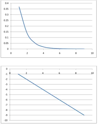
13 Mathematical Basics Ϭ Ϭ͘Ϭϱ Ϭ͘ϭ Ϭ͘ϭϱ Ϭ͘Ϯ Ϭ͘Ϯϱ Ϭ͘ϯ Ϭ͘ϯϱ Ϭ͘ϰ Ϭ Ϯ ϰ ϲ ϴ ϭϬ ͲϭϬ Ͳϵ Ͳϴ Ͳϳ Ͳϲ Ͳϱ Ͳϰ Ͳϯ ͲϮ Ͳϭ Ϭ Ϭ Ϯ ϰ ϲ ϴ ϭϬ

Figure 1.1: Linearization of an exponential (top) by plotting the logarithm (bottom) (Plots were prepared using Microsoft Excel (MS Office 2007))

Any function can be linearized if you use the Taylor series expansion given as:

ݕሺݔͲ൅ ݔሻ ൌ ݕሺݔͲሻ ൅ ቀ݀ݕ_݀ݔቁ_ݔ ݋ή ሺݔ െ ݔͲሻ ൅ ͳ ʹǨή ቀ ݀ʹ_ݕ ݀ݔʹቁ_ݔ ݋ ή ሺݔ െ ݔͲሻ ʹ_൅ͳ ͵Ǩή ቀ ݀͵_ݕ ݀ݔ͵ቁ_ݔ ݋ ή ሺݔ െ ݔͲሻ

͵_{൅ ڮ}_(Eq.1.32)

One important (and the only!) example for a Taylor series expansion we use in this textbook concerns the logarithm, i.e.:

ሺͳ െ ݔሻ ൌ ͳ ൅ ቀ_ͳെݔെͳቁ ݔ݋ൌͲή ሺݔ െ Ͳሻ ൅ ͳ ʹǨή ቀ െͳ ሺͳെݔሻʹቁ ݔ݋ൌͲή ሺݔ െ Ͳሻ ʹ_{൅ ڮ ൎ െݔ} (Eq.1.33)

(14)

1.4

Treating experimental data – SI-system and error calculation

(A) Units – the SI-system:

The standard system of physical units (system international (French), SI) contains only a limited number, namely kg (kilogram) for mass, m (meter) for length, s (second) for time, A (Ampere) for charge per time (= electric current), and K (Kelvin) for (absolute) temperature. All other units can be expressed in terms of these basic units, and any student of science should be capable of this, since it comes in handy in (i) deriving simple formulae, (ii) understanding physical quantities, and (iii) calculating quantities based on certain variables. As one important example, let us consider several ways of expressing energy:

1) potential energy equals force times length, and force is acceleration times mass, therefore energy should be: kg m s-2_{m = kg m}2_s-2_{= J (Joule)}

2) alternatively, energy is power times time, therefore W s (or, not SI, but more common: kWh) 3) in electrostatics, energy is voltage times charge, therefore A s V (or keV (kilo electron Volt,

not SI, with the elementary charge 1 e = 1.6 10-19_{A s))}

The most common derived SI units are: N (Newton) for force, Pa (Pascal) for pressure, J (Joule) for energy, W (Watt) for power, C (Coulomb) for electric charge, V (Volt) for voltage, Ω (Ohm) for electric resistance.

(B) Error calculation:

Experimental data are not perfect, that is, even if you repeat a given experiment several times, you will get at least slightly different results. If x₁, x₂, x₃, ….., x_N is a set of these different results obtained from a total of N single measurements, these data are evaluated as following:

First, one has to calculate the average of the experimental quantity x, i.e.

ۃݔۄ ൌ_ܰͳσܰ݅ൌͳݔ݅ (Eq.1.34)

To determine the reliability of this average, we then have to calculate the standard deviation. The apparent error of a single experiment is given as οݔ_݅ ൌ ۃݔۄ െ ݔ_݅ and the standard deviation then is obtained by averaging the absolute values of all apparent errors, i.e.

ܵ ൌ ටσܰ݅ൌͳοݔ݅ʹ

ܰെͳ , with N > 1 (Eq. 1.35)

(15)

Click on the ad to read more Basic Physical Chemistry

15

Mathematical Basics

Within a written report of the experiment, the result must then be given as ݔ ൌ ۃݔۄ േ οݔ, providing both the average and the reliability.

(C) Error progression:

In most experiments, a given physical quantity depending on several individually measured parameters has to be calculated. As one example, let us consider a quantity z depending on two parameters x, y, that is ݖ ൌ ݂ሺݔǡ ݕሻ. In this case, the calculated error of z depends on the statistical errors of the two physical parameters x, y as following (error progression):

οݖ ൌ ቀ݀ݖ_݀ݔቁ

ۃݔۄǡۃݕۄή οݔ ൅ ቀ ݀ݖ

݀ݕቁ_{ۃݔۄǡۃݕۄ}ή οݕ (Eq.1.37)

Note that the derivatives could be positive or negative, and therefore partially compensate each other, which does not make much sense. Therefore, one has to calculate the absolute values, i.e.

οݖʹ _{ൌ ቀ}݀ݖ ݀ݔቁ_{ۃݔۄǡۃݕۄ}

ʹ

ή οݔ ൅ ቀ݀ݖ_݀ݕቁ

ۃݔۄǡۃݕۄ ʹ

ή οݕ (Eq.1.38)

or

οݖ ൌ ඨቀ_݀ݔ݀ݖቁ

ۃݔۄǡۃݕۄ ʹ

ή οݔ ൅ ቀ_݀ݕ݀ݖቁ

ۃݔۄǡۃݕۄ ʹ

ή οݕ (Eq.1.39)

Linköping University –

innovative, highly ranked,

European

Interested in Engineering and its various branches? Kick-start your career with an English-taught master’s degree.

(16)

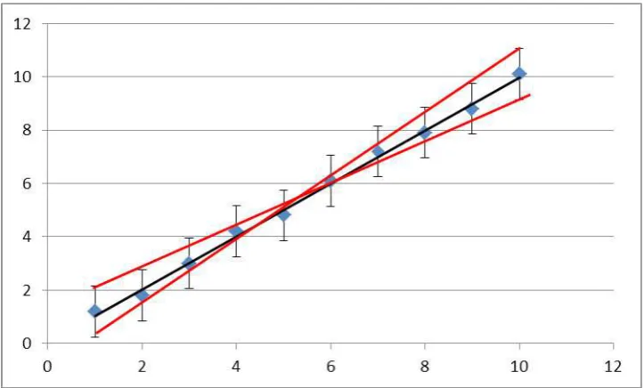
As we have seen before, often physical-chemical data are represented in a linear relation, and the intercept and the slope provide the quantities of interest. To determine the error of this linear analysis, formally linear regression has to be used. This requires plugging all of your individual data points into the computer, and trusting the numerical calculation of the errors of intercept and slope. Additionally simple linear regression might ignore the statistical errors of individual data points. In practice the following approach is much more convenient and reliable.

First, plot all your data points considering the statistical errors of each individual point (= error bars), respectively. 2nd_{, draw two extreme lines which contain all data points with error bars, as well as an}

intermediate line. From this simple picture, you then can determine average slope and intercept, as well as the error of these two. The procedure is illustrated in figure 2.

(17)

17

Thermodynamics

2 Thermodynamics

Phenomenological thermodynamics is mainly concerned with equations and variables of state, energy exchange at physicochemical processes, and phase- and chemical equilibrium. The goal of this chapter is to give a complete overview of all important concepts used in phenomenological thermodynamics, and provide some illustrative examples when appropriate.

We will start with some basic definitions concerning physico-chemical systems and processes, then introduce the ideal and real gas equations of state, and finally discuss the fundamental principles of thermodynamics. Here, physical models for the heat capacity of ideal gases and solids will allow us to calculate the energy, heat and work exchange for any given process, even cycles such as the Carnot process.

Next, the phase equilibrium of both pure components and binary mixtures will be addressed. For the latter, in the case of high dilution, simple formula for so-called colligative phenomena such as lowering of the freezing temperature, increase of the evaporation temperature, or osmotic pressure will be derived and discussed. Finally, we will talk about the equilibrium of chemical reactions, as well as about energetic aspects of chemical reactions.

2.1 Definitions

In thermodynamics, systems are classified according to their ability to exchange matter and/or energy with their environment:

RSHQ FORVHG LVRODWHG

(18)

An example for an open system, which can exchange both matter and energy with the environment, is an open beaker filled with boiling water (heat is lost to the environment, and matter is lost due to evaporation of water), whereas an example for a closed system would be a pot of boiling water tightly closed with a lid (only heat is lost). An isolated system would be, for instance, a closed thermostat bottle filled with hot tea: neither energy nor matter is exchanged with the environment.

On the other hand, physico-chemical processes are classified as following: 1. Isochor, i.e. the volume of the system is kept constant (dV = 0), 2. Isobar, i.e. the pressure is kept constant (dp = 0), 3. Isotherm, i.e. the temperature is kept constant (dT = 0), or 4. Adiabatic, i.e. no exchange of heat with the environment (Q = 0).

Finally, we have to consider the different aggregate states of matter: solid (defined volume and shape), liquid (defined volume, undefined shape), and gas (neither volume nor shape is defined)

as a

e

s

al na

eal responsibili�

I joined MITAS because

Maersk.com/Mitas

�e Graduate Programme for Engineers and Geoscientists

as a

e

s

al na or o

Month 16

I was a construction

supervisor in

the North Sea

advising and

helping foremen

solve problems

I was a

he

s

Real work International opportunities �ree work placements

al Internationa or �ree wo al na or o

I wanted real responsibili�

I joined MITAS because

(19)

19

Thermodynamics

2.2

Gas equations

2.2.1 The ideal gas

In 1679, Boyle and Mariotte found experimentally that for a gas undergoing an isothermal process (either compression or expansion) its volume times its pressure remain constant:

݌ ή ܸ ൌ ܿ݋݊ݏݐ (Eq.2.1)

, namely 22.12 l bar for 1 mole gas at temperature t = 0 °C.

In 1800, Gay-Lussac discovered that for isobaric or isochoric processes, the volume or the pressure of a gas, respectively, increases linearly with temperature:

1st_{law of Gay-Lussac:} ܸ ൌ ܸ

Ͳή ሺͳ ൅ ߙͲή ݐሻ (Eq.2.2)

Here,ܸ_Ͳ is the volume of the gas at standard conditions (p = 1.013 bar, t = 0°C). Importantly, different gases all have the same normalized thermal expansion coefficient:

ߙͲൌቀ

οܸ οݐቁ

ܸͲ ൌ

ͳ

ʹ͹͵Ǥͳ͸ιܥ (Eq.2.3)

, and we obtain therefore:

ܸ ൌ ܸͲή ቀͳ ൅_ʹ͹͵Ǥͳ͸ݐ ቁ ൌ ܸͲή ቀʹ͹͵Ǥͳ͸൅ݐ_ʹ͹͵Ǥͳ͸ ቁ ൌ ܸͲή ߙͲή ܶ (Eq.2.4)

Here, T is a new temperature scale with unit “Kelvin”. Both scales can simply be converted into each other according to ܶ ሾܭሿΤ ൌ ݐ ሾιܥሿ ൅ ʹ͹͵Ǥͳ͸Τ Note that, for the description of the isochoric processes of the ideal gas the Kelvin scale is more convenient, since simple proportionality is obtained. Also, since no negative volume can exist, it is obvious that T = 0 K (or t = – 273.16 °C) is the smallest temperature possible. Therefore, the Kelvin scale is also called the scale of absolute temperature, whereas the Celsius scale is based on the properties of one specific chemical, water, which freezes under standard pressure at t = 0 °C, and boils at 100 °C.

For the isochoric process, in analogy the 2nd_{law of Gay-Lussac can be formulated:}

2nd_{law of Gay-Lussac:} ݌ ൌ ݌

Ͳή ሺͳ ൅ ߚͲή ݐሻ (Eq.2.5)

Here, ݌଴ is the pressure of the gas at standard conditions (p = 1.013 bar, t = 0°C). Importantly, again different gases all have the same normalized thermal compressibility coefficient:

ߚͲ ൌ ቀο݌_οݐቁ

݌Ͳ ൌ

ͳ

(20)

and we obtain therefore:

݌ ൌ ݌Ͳή ቀͳ ൅_ʹ͹͵Ǥͳ͸ݐ ቁ ൌ ݌Ͳή ቀʹ͹͵Ǥͳ͸൅ݐ_ʹ͹͵Ǥͳ͸ ቁ ൌ ݌Ͳή ߚͲή ܶ (Eq.2.7)

To obtain the general equation of state of the ideal gas irrespective of the process, we next combine the laws of Boyle, Mariotte and Gay-Lussac, using formally a two-step process to change from a given set of state variables ሺ݌_Ͳǡ ܸ_Ͳǡ ܶ_Ͳሻ to a completely different set of variablesሺ݌_ͳǡ ܸ_ͳǡ ܶ_ͳሻ:

ሺ݌Ͳǡ ܸͲǡ ܶͲሻ݀ܶൌͲሱۛۛሮ ሺ݌ͳǡ ܸݔǡ ܶͲሻ݀݌ ൌͲሱۛۛሮ ሺ݌ͳǡ ܸͳǡ ܶͳሻ (Eq.2.8)

For the first isotherm step we use the law of Boyle, Mariotte to express the unknown volume ܸ_ݔ:

݌ͳή ܸݔ ൌ ݌Ͳή ܸͲ ՜ ܸݔ ൌ ܸͲή݌_݌Ͳ_ͳ (Eq.2.9)

For the 2nd_{isobar step we used the first law of Gay-Lussac, i.e.:}

ܸ̱ܶ ՜ ܸͳ

ܶͳ ൌ

ܸݔ

ܶͲ ՜ ܸݔ ൌ

ܸͳ

ܶͳή ܶͲ (Eq.2.10)

We then can replace ܸ_ݔ in (Eq.2.9), and finally obtain:

ܸͳ

ܶͳή ܶͲൌ ܸͲή

݌Ͳ

݌ͳ ՜

݌ͳήܸͳ

ܶͳ ൌ

݌ͲήܸͲ

ܶͲ (Eq.2.11)

Since our starting conditions “0” as well as our final state “1” have been chosen arbitrarily, we can conclude that:

݌ͳήܸͳ

ܶͳ ൌ ܿ݋݊ݏݐ (Eq.2.12)

According to experimental observations, this constant is given by the amount of gas in mole n, and the universal gas constant = 8.314 J/(mole K), and one obtains the universal law of ideal gases:

(21)

Click on the ad to read more Basic Physical Chemistry

21

Thermodynamics

([DPSOH

&RQVLGHU D VPDOO ODE P _{DUHD KHLJKW P ZKHUH DQ DXWRPDWLF &2}

ILUH H[WLQJXLVKHU

GXULQJDVXGGHQILUHLQRQHRIWKHKRRGVVXGGHQO\UHOHDVHVNJRI&2:KDWLVWKHHIIHFWLYH

PDVVSHUP_{DFWLQJRQWKHZLQGRZVRIWKHODEGXHWRWKHVXGGHQO\LQFUHDVHGSUHVVXUHXVHWKH}

LGHDOJDVHTXDWLRQRIVWDWHIRUDSSUR[LPDWLRQ"

6ROXWLRQ7KHNJRI&2 0 J0ROFRUUHVSRQGWR 0ROJDV7KH

FRUUHVSRQGLQJDGGLWLRQDOSUHVVXUHWKHUHIRUHLV

݌ܥܱʹ ൌ

݊ήܴήܶ ܸ ൌ

ʹʹ͹Ǥ͵ήͺǤ͵ͳͶήʹͻ͵

ʹͲή͵ ܲܽ ൌ ͻʹʹͺܲܽ ൌ ͻʹʹͺ

ܰ ݉ʹ

7KHHIIHFWLYHDGGLWLRQDOPDVVSHUP_{FRUUHVSRQGLQJWRWKLVH[FHVVSUHVVXUHLVWKHQJLYHQE\}

ܨ ൌ ݉ ή ݃ ! ͻʹʹͺܰ ൌ ݉ ή ͻǤͺͳ_݇݃ܰ ! P NJ

7KHUHIRUH QHDUO\ WRQ DFWVRQ P _{RI RXU ODE ZLQGRZV VR PRVW OLNHO\ WKH ZLQGRZV ZLOO}

(22)

Note that the ideal gas law (Eq.2.13) should be considered as a phenomenological law which is confirmed by experience, but it provides no explanation in terms of microscopic molecular motions. In the next section “kinetic gas theory” we will therefore discuss the ideal gas based on a microscopic single particle-based description developed by Maxwell, Boltzmann and others in the 19th_century.

2.2.2 Kinetic Gas Theory

For the microscopic description of the ideal gas, we consider particles with mass m but no volume, which move without interactions in a strictly ballistic way between the rigid walls of a cubic sample container with side length a. Further, the number of gas particles is very large, so we can apply Boltzmann statistics. Note that a detailed derivation of the Boltzmann distribution is beyond the scope of this book, so we refer the reader to any common text book, section “statistical thermodynamics”.

For this ideal gas system, the velocity distribution as a function of sample temperature and single gas particle mass m is then given, according to Maxwell and Boltzmann, as:

݂ሺݑሻ ؆ ቀ_ʹ݇݉

ܤܶቁ

ͳǤͷ

ή ݑʹ_{ή ቂെ}݉ൗ ήݑʹ ʹ

݇ܤܶ ቃ (Eq.2.14)

It should be noted here that the exponential in this expression corresponds to the Boltzmann factor. Here, the Boltzmann constant is given as ݇_ܤ ൌ ͳǤ͵ͺ ή ͳͲെʹ͵ܬ ݏΤ According to the Boltzmann factor, states of lower energy have a higher statistical probability of being occupied by the particles, as shown in figure 2.2. Multiplying this factor with the term ݑʹ, which is introduced in Eq.(2.14) due to a spatial integral over all possible directions of particle motion, one obtains a maximum velocity, which in dependence of temperature is shifted to higher values (see figure 2.3).

ܶ ൌ Ͳܭǡܰͳൌ ܰ ܶ ൌ οܧ ݇Τ ǡܰͳൌ ͲǤ͹͵ܰ ܶ ՜ λǡܰͳ ൌ ܰʹൌ ܰ ʹΤ

Fig. 2.2.: Boltzmann distribution at different T, 2-state-system

In general, the ratio of occupation probability of an energetically excited state ܰ_ʹ compared to the occupation probability of the ground state ܰ_ͳ according to the Boltzmann factor depends on temperature and energy difference ܧ_ʹെ ܧ_ͳൌ οܧ as:

ܰʹ

ܰͳ ൌ ቂെ

ܧʹെܧͳ

݇ܤܶ ቃ ൌ ቂെ

οܧ

(23)

23

Thermodynamics

Contrary to Fig. 2.2., our ideal gas particles in principle can assume any velocity and not just a quantized set of discrete values. However, the Boltzmann factor itself is not necessarily restricted to quantized energy states, but describes any probability ratio of populations ܰʹ

ܰͳ separated in energy by οܧ

We will meet this extremely important concept of the Boltzmann factor more frequently throughout this book. Here, let me just name one analogous example from kinetics, the well-known Arrhenius-equation:

݇ ൌ ή ቂെ ܧܣ

݇ܤܶቃ (Eq.2.16)

with k the reaction velocity constant, and ܧ_ܣ the energy of activation. The exponential term here describes the probability to reach the excited state via thermal excitation at temperature T.

Coming back to our ideal gas treated on a microscopic level, let us discuss the shape of the Maxwell-Boltzmann velocity distribution at different temperatures in more detail:

u

f(u)

Fig. 2.3.: Maxwell-Boltzmann velocity distribution at different temperatures (from cold (blue) to hot (red))

(24)

The expression for the velocity distribution (Eq.2.14) allows us to calculate an analytical expression of the average squared velocity of a single particle as a function of sample temperature. We also need a relation between this average squared velocity and the macroscopic pressure to discuss the equation of state of the ideal gas in terms of microscopic molecular motions. Pressure is force per area, and force is the time derivative of the momentum, which itself is mass times velocity. Therefore, the pressure enacted by a single gas particle colliding with one wall of our cubic box is given as:

݌ ൌܨ_ܣൌቀ݀ሺ݉ ήݑݔሻ݀ݐ ቁ

ܽݔ ʹ (Eq.2.17)

The momentum of this particle is only changed at the collision, where it is reverted. Further, the time between two collisions is given by the velocity and the distance, and we therefore can express the momentum change with time as:

ቀ݀ሺ݉ήݑݔሻ

݀ݐ ቁ ൌ

οሺ݉ήݑݔሻ

οݐ ൌ

݉ήݑݔെെ݉ήݑݔ

ʹή݈ݔΤݑݔ ൌ

݉ήݑݔʹ

݈ݔ (Eq.2.18)

For all particles within our cubic box, the overall momentum transfer related to the pressure is given by summing up the individual effects and replacing the squared velocity of the single particle with the average quantity:

݌ ൌܨ_ܣൌσ

݉ήۃݑݔʹۄ

݈ݔ

݈ݔʹ

൙ ൌ ܰ ή݉ήۃݑݔʹۄ

(25)

25

Thermodynamics

or

݌ ή ܸ ൌ ܰ ή ݉ ή ۃݑݔʹۄ (Eq.2.20)

Since all directions x, y and z have the same probability, the average squared velocity in 3d is given as

ۃݑʹ_{ۄ ൌ ۃݑ}

ݔʹۄ ൅ ۃݑݕʹۄ ൅ ۃݑݖʹۄ ൌͳ_͵ή ۃݑݔʹۄ (Eq.2.21)

leading to

݌ ή ܸ ൌ ܰ ή ݉ ήۃݑ_͵ʹۄ (Eq.2.22)

According to the Maxwell-Boltzmann distribution (Eq.(2.14)), the average squared velocity of the particles can be calculated, corresponding to an average kinetic energy per particle of

ͳ

ʹή ݉ ή ۃݑʹۄ ൌ ͵

ʹή ݇ܤή ܶ (Eq.2.23)

Therefore, for a total number of gas particles ܰ_ܣൌ ͸ǤͲʹ ή ͳͲʹ͵, we obtain:

݌ ή ܸ ൌ ܰ ή ݉ ήۃݑ_͵ʹۄൌ ܰܣή ݇ܤή ܶ ൌ ܴ ή ܶ (Eq.2.24)

with the gas constant given as ܴ ൌ ܰ_ܣή ݇_ܤ ൌ ͺǤ͵ͳͶ ܬ ሺ݉݋݈݁ ή ܭሻΤ !

([DPSOH

&DOFXODWHWKHPHDQVTXDUHGYHORFLW\RIQLWURJHQPROHFXOHVDWURRPWHPSHUDWXUHDQGFRPSDUH \RXUUHVXOWWRWKHYHORFLW\RIVRXQG

6ROXWLRQ:HVLPSO\XVHWKHPDVVSHUPROHFXOHP J1$DQGWKHIROORZLQJH[SUHVVLRQ

ͳ

ʹή ݉ ή ۃݑʹۄ ൌ ͵

ʹή ݇ܤή ܶ ! ۃݑʹۄ ൌ ͵ή݇ܤήܶ

݉ ൌ

͵ήͳǤ͵ͺήͳͲെʹ͵_ήʹͻ͵

ͲǤͲʹͺ ͸ǤͲʹήͳͲ_Τ ʹ͵

݉ʹ

ݏʹ ൌ ʹ͸Ͳ͹ͻͻ

݉ʹ

ݏʹ

7KHUHIRUHWKHPHDQYHORFLW\LV

ඥۃݑʹ_{ۄ ൌ ξʹ͸Ͳ͹ͻͻ}݉

ݏ ൌ ͷͳͲǤ͹ ݉

ݏ

(26)

2.2.3 Real Gases, isotherms and critical conditions

For ideal gases, we ignored the particle volume as well as interparticle interactions, whereas in reality gas particles are molecules or atoms which possess both characteristics. The interactive forces are either caused by permanent dipoles or by fluctuating dipoles which depend on polarizability of a given molecule. For example, in the case of noble gases the fluctuating dipoles increase from He to Xe resulting in greater strength of attractive forces. To take these effects into account, we reformulate the ideal gas equation of state into the so-called Van-der-Waals-equation:

ቀ݌ ൅݊_ܸʹʹήܽቁ ή ቀܸ_݊െ ܾቁ ൌ ሺ݌ ൅ ߨሻ ή ቀܸ_݊െ ܾቁ ൌ ܴ ή ܶ (Eq.2.25 a)

or, with ݒ ൌܸ

݊ the molar volume:

ቀ݌ ൅_ݒܽʹቁ ή ሺݒ െ ܾሻ ൌ ሺ݌ ൅ ߨሻ ή ሺݒ െ ܾሻ ൌ ܴ ή ܶ (Eq.2.25 b)

Note that the pressure the real gas enacts on the wall of a container, compared to the ideal gas, is reduced due to the attractive forces, i.e.

݌

_ݎ݁

ൌ ݌

_݅݀

െ ߨ ൏ ݌

_݅݀, whereas the sample volume itself is

increased by the molar particle volume, i.e.

ݒ

_ݎ݁

ൌ ݒ

_݅݀

൅ ܾ ൐ ݒ

_݅݀

If you compare the ideal gas and the real gas laws at identical ܴ ή ܶ

this means that: (i) the external pressure to keep the volume of the ideal gas constant has to be higher than in case of the real gas, and (ii) at given container volume V the sample volume accessible by the gas particles is larger for ideal gases than for real gases. The excluded volume b corresponds effectively to a short-range repulsive interparticle interaction. For spherical gas particles, like noble gas atoms, it can be simply calculated from the single particle volume according to the following sketch:

(27)

Click on the ad to read more Basic Physical Chemistry

27

Thermodynamics

In Fig. 2.3., the dotted circle corresponds to the excluded spherical volume which contains only a single particle at once. This volume is defined by two spherical particles at closest contact, and therefore has a radius of twice the single particle radius, and correspondingly eight times the single particle volume. In conclusion, since the sketch holds for two particles which exclude each other, the excluded volume per single particle corresponds to four times the particle volume, i.e. ܾ ൌ Ͷ ή ܸ_ܣݐ݋݉

The overall interaction between two real gas particles is described by the interaction pair potential sketched in figure 2.4. or

ܧሺߪሻ ൌ Ͷ ή ߝ ή ൤ቀߪ݉

ߪ ቁ ͳʹ

െ ቀߪ݉

ߪ ቁ ͸

൨ (Eq.2.26)

89,000 km

In the past four years we have drilled

That’s more than twice around the world.

careers.slb.com

What will you be?

Who are we?

We are the world’s largest oilfield services company1_.

Working globally—often in remote and challenging locations— we invent, design, engineer, and apply technology to help our customers find and produce oil and gas safely.

Who are we looking for?

Every year, we need thousands of graduates to begin dynamic careers in the following domains:

n Engineering, Research and Operations

n Geoscience and Petrotechnical

(28)

In Fig. 2.4., the parameter σ_m corresponds to the interparticle distance σ where attractive and repulsive interaction energy compensate exactly, whereas the minimum position in the figure corresponds to the stable state with maximum net attraction. Therefore, σ_m is a measure of the particle size of excluded volume (see van-der-Waals-Eq.). Note that the depth of this minimum is parameterized by ε. This parameter therefore provides a measure for the attractive interparticle forces or the internal pressure of the van-der-Waals-Eq. In the Eq.(2.26), one should also note that the attractive interaction energy based on dipole-dipole-attraction scales with inverse interparticle distance to the power of 6, whereas the repulsive interaction caused by direct overlap of the electron clouds of neighboring particles has a much shorter range and scales with inverse interparticle distance to the power of 12. Here, one should recall that the attractive Coulomb interaction energy between a positive and a negative charge scales with 1/σ, and therefore has a much longer range than dipole-dipole-attraction.

ܧሺߪሻ

ߪ

Fig. 2.4.: Interaction pair potential of real gas particles

(29)

29

Thermodynamics

Fig. 2.5.: Isotherms of a real gas above, at and below the critical temperature (from: Gerd Wedler und Hans-Joachim Freund, Lehrbuch der Physikalische Chemie, p. 271, 6.Auflage, Weinheim 2012. Copyright Wiley-VCH Verlag GmbH & Co. KGaA. Reproduced with permission.)

(30)

Once we reach point B, all material has become liquid, and due to the low incompressibility of the condensed phase the pressure now has to increase strongly if we try to further decrease the sample volume. Here, it is important that the experimental horizontal connecting the pure liquid at B with the pure gas at A can be constructed from the van-der-Waals-curve by keeping the area below the two different curves, which corresponds to the overall work, identical. This is obvious since the energy change of the system from point A to point B corresponding to the condensation heat has to be independent of the process itself. At temperatures above the critical temperature, this condensation is not possible any longer, and there is no difference between gas and liquid.

The macroscopic variables of state of the critical point, ሺ݌_ܭǡ ܸ_ܭǡ ܶ_ܭሻ, can be expressed as simple functions of the microscopic variables of the Van-der-Waals-Eq.ሺܽǡ ܾሻ and vice versa, if you consider that within the isotherm at ܶ ൌ ܶ_ܭ it is a turning point with slope zero. Therefore, the first and second derivative of ݌ሺܸሻ have to be zero, that is,

ቀ݀݌_ܸ݀ቁ

ܸܭǡܶܭ ൌ ቀ

݀ʹ_݌

ܸ݀ʹቁ_ܸ

ܭǡܶܭ ൌ Ͳ

(Eq.2.27)

“The perfect start

of a successful,

international career.”

CLICK HERE

to discover why both socially and academically the University

of Groningen is one of the best places for a student to be

www.rug.nl/feb/education

(31)

31

Thermodynamics

Solving the Van-der-Waals-Eq. and using, in addition, these derivatives, one obtains the following relations between the microscopic van-der-Waals-parameters of a real gas and its critical point:

ܾ ൌͳ_͵ή ܸܭ (Eq.2.28)

ܽ ൌͻ_ͺή ܴ ή ܶܭή ܸܭ (Eq.2.29)

݌ܭ ൌ͵_ͺή ܴ ήܶ_ܸܭ_ܭ ൌ_͵ήܾܽʹ (Eq.2.30)

(32)

2.3

The fundamental laws of thermodynamics

2.3.1 Definition of temperature

If two systems A and B coexist in thermal equilibrium, and also B is in thermal equilibrium with a 3rd

system C, then all three systems are in thermal equilibrium and have the same temperature. This simple principle is the basis for temperature measurements as well as one foundation of phase equilibrium and chemical equilibrium.

2.3.2 The first law of thermodynamics

The first law of thermodynamics is the law of conservation of energy including, in contrast to conventional physics, heat as an additional means of energy exchange between system and environment. It is formulated for differential changes or measurable changes in total energy U, respectively, as:

ܷ݀ ൌ ߜܳ ൅ ߜܹ ڮοܷ ൌ ܳ ൅ ܹ (Eq.2.31)

with U the internal energy, Q the heat flow, and W the work, i.e. typically volume work (expansion or compression). To define the heat flow, we refer to adiabatic processes, where the system is thermally isolated from its environment, and therefore οܷ_{ሺܽ݀ ሻ} ൌ ܳ ൅ ܹ ൌ ܹ_{ሺܽ݀ ሻ} therefore ܳ ൌ െܹ ൅ ܹ_{ሺܽ݀ ሻ} Note that heat and work are not quantities of state, in contrast to U, but depend on the process itself, whereas

οܷ

only depends on the final and the initial state. As a consequence, Q and W also are not total differentials, but have to be formulated as or _ߜ

ܳ

RU_ߜ

ܹ

respectively. In experimental practice,

οܷ

becomes important for processes at constant volume (isochors), since then it corresponds directly to the heat exchange between system and environment. On the other hand, for isobaric processes the heat transfer corresponds to the enthalpy change

οܪ

ܪ ൌ ܷ ൅ ݌ܸ, see Eq.(2.33)):

isochors: ߜܹ ൌ Ͳ ՜ ܷ݀ ൌ ߜܳ ൌ ܿ_ܸ ή ݀ܶ (Eq.2.32)

isobars: ߜܹ ൌ െ݌ܸ݀ ൌ െܴ݀ܶ ՜ ݀ܪ ൌ ݀ሺܷ ൅ ݌ܸሻ ൌ ߜܳ ൌ ܿ_݌ή ݀ܶ (Eq.2.33)

For illustration, let us consider these two processes with a system of 1 mole ideal gas. Note that, at given heat exchange Q, the temperature effect οܶ will be larger in case of the isochoric process, since in case of the isobaric part of the energy will be lost due to volume expansion work. As a consequence, the heat capacity ܿ_ܸ has to be smaller than ܿ_݌ namely ܿ_݌െ ܿ_ܸ ൌ ܴ for 1 Mol ideal gas.

Importantly, for the ideal gas the energy change for isothermal processes is zero, i.e. in general:

ܷ݀ ൌ ߜܳ ൅ ߜܹ ൌ ܸܿ݀ܶ ൌ Ͳ (Eq.2.34)

(33)

Click on the ad to read more Basic Physical Chemistry

33

Thermodynamics

For 1 mole ideal gas, this work can be calculated as:

ܹ݀ ൌ െ݌ܸ݀ ൌ െܴܶ_ܸ ܸ݀ ՜ ܹ ൌ െ ׬ ܴܶ_ܸ ܸ݀ ൌ െܴܶ ή ቀܸʹ

ܸͳቁ

ܸʹ

ܸͳ (Eq.2.35)

In contrast, for real gases one also has to take into account the internal work versus the attractive interparticle interactions, and the total internal energy change is given as:

ܷ݀ ൌ ܸܿ݀ܶ ൅ ߨܸ݀ ൌ Ͳ (Eq.2.36)

Therefore, if a real gas is expanding into vacuum, both heat exchange (Q), volume work (W) and, as a consequence of the first law of thermodynamics, the overall change in internal energy

οܷ

are all zero. The temperature will thus drop to compensate for the internal work ߨܸ݀

(Joule’s experiment).

Finally, let us finish our discussion of the first law of thermodynamics in the context of ideal gas processes with the adiabatic process. Here, the first law will allow us a very simple derivation of an equation of state for adiabatic processes, which will come in handy in the next section about the 2nd_{law of thermodynamics.}

For adiabatic processes of 1 Mol ideal gas the first law reads as following:

ܷ݀ ൌ ߜܳ ൅ ߜܹ ൌ Ͳ െ ݌ܸ݀ ൌ ܸܿ݀ܶ ൌ ߜܹܽ݀ (Eq.2.37)

AXA Global

Graduate Program

(34)

To derive our equation of state, we insert the ideal gas law for p, and obtain:

െܴܶ_ܸ ܸ݀ ൌ ܸܿ݀ܶ (Eq.2.38)

െܸ݀_ܸ ൌܸܿ

ܴ ݀ܶ (Eq.2.39)

Integration of this differential with finite boundaries (T₁,V₁) as initial and (T₂,V₂) as final state yields

െ ቀܸʹ

ܸͳቁ ൌ

ܸܿ

ܴ ቀ ܶʹ

ܶͳቁ (Eq.2.40)

Or

ܸͳή ܶͳܸܿΤܴൌ ܸʹή ܶʹܸܿΤܴ ൌ ܿ݋݊ݏݐ (Eq.2.41)

If you apply the ideal gas law to replace T with p, and consider that for one mole ideal gas ܿ_݌െ ܿ_ܸ ൌ ܴ then,

݌ ή ܸܿ݌Τܸܿ _{ൌ ܿ݋݊ݏݐ}_(Eq.2.42)

This is our equation of state for an adiabatic process, expansion or compression, of the ideal gas, allowing us to calculate any missing variable of state.

Comparing this equation with the equation of state for the isotherm of an ideal gas (Boyle’s law:

݌ ή ܸ ൌ ܿ݋݊ݏݐ, we expect at identical volume expansion from identical initial states that the adiabatic

p(V) drops more in pressure than the isotherm, i.e. that also the temperature is lowered, since in this case the expansion volume work is not compensated by heat exchange.

2.3.3 The 2nd_{law of thermodynamics and the Carnot process}

Whereas the first law deals with the energy, the 2nd_{law of thermodynamics is concerned with a new}

quantity of state, the entropy. We should note that in thermodynamics “order” is not just spatial order in the usual 3-dim space. It rather refers to a “phase space” which includes momentum (velocity) coordinates. For example, in an ideal gas, the spatial ordering of molecules is independent of temperature at constant volume. However, the “order” in velocity space decreases with increasing temperature (and increasing average molecular velocity in a gas) resulting in an increase of entropy. Quantitatively and macroscopically, entropy is defined as the reversibly exchanged amount of heat between system and environment at given temperature T

݀ܵ ൌ݀ܳݎ݁ݒ

ܶ ՜ οܵ ൌ

ܳݎ݁ݒ

(35)

35

Thermodynamics

This means that dU=TdS – dW_rev, and we will show later that the reversible work is the maximum you can get, as a theoretical limit. Eq.2.43 is the first part of the 2nd_{law of thermodynamics, defining the change}

in entropy as a new fundamental quantity valid for strictly reversible processes.

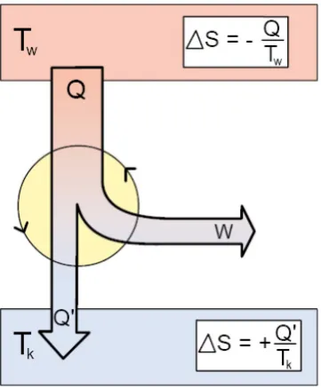
To discuss the maximum work one can extract from a reversible cyclic process, we next consider the famous Carnot process as a reference. This process describes an ideal reversible and therefore hypothetic machine partially transferring heat into work. The principle is illustrated in figure 2.7.

Fig. 2.7.: thermodynamic machines – principle of the Carnot process

This machine is based on the reversible heat flow from a reservoir with higher temperature T_w to a reservoir with colder temperature T_k. Note that both reservoirs are considered to be infinitely large, so their temperature will not change during the process. Importantly, the amount of heat transferred to the colder reservoir Q’ is smaller than the amount of heating taken from the hot one Q, and the difference W = Q – Q’ can be used a volume expansion work. Note that the overall entropy change for this reversible process is zero, i.e.

οܵݐ݋ݐ ൌ െ_ܶܳ_ݓ൅_ܶܳԢ_݇ ൌ Ͳ (Eq.2.44)

If we are running our machine in reverse direction, which should not change the respective amounts of heat and work, since the process is perfectly reversible, we obtain a so-called heat pump, which transfers heat from cold to warm upon work input, in the reverse direction compared to the spontaneous heat flow.

The efficiency of this type of machine transferring heat into work is defined as the ratio of work output over heat input, i.e.

ߟ ൌܹ_ܳ ൌܶݓെܶ݇

(36)

Only if T_k = 0, a limit which according to the 3rd_{law of thermodynamics (see section 2.3.5.) can never be}

reached in practice, the efficiency of our machine may reach one. In general, one cannot transfer heat Q into work W without loss, and the highest efficiency possible is given by the reversible machine, a limit which can never be reached in practice. Note that, in accordance with energy conservation, it could be possible to transfer heat into work directly. However, the 2nd_{law tells us that this cannot be achieved:}

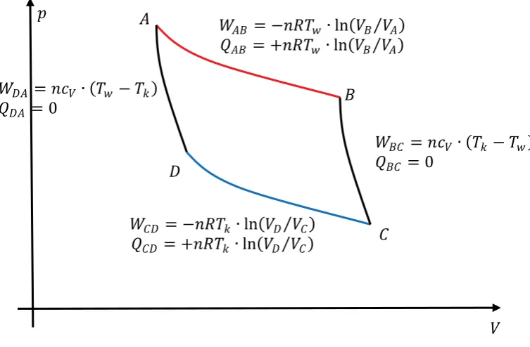
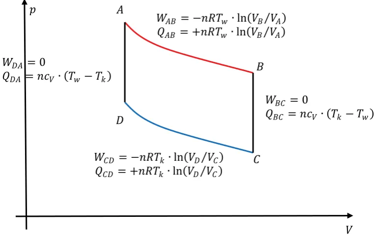
meaning that heat somehow is a worse form of energy compared to work from a practical point of view. This is directly related to entropy, as we will see. First, let us derive the above formula describing our limit in heat-work conversion efficiency by discussion of the Carnot process in more detail. This hypothetical ideal circular process is based on isothermal and adiabatic expansions and compressions, as shown in figure 2.8.

ܣ

ܤ

ܥ

ܦ

݌

ܸ

ܹ

ܣܤ

ൌ െܴ݊ܶ

ݓ

ή ሺܸ

ܤ

Τ ሻ

ܸ

ܣ

ܳ

ܣܤ

ൌ ൅ܴ݊ܶ

ݓ

ή ሺܸ

ܤ

Τ ሻ

ܸ

ܣ

ܹ

ܥܦ

ൌ െܴ݊ܶ

݇

ή ሺܸ

ܦ

Τ ሻ

ܸ

ܥ

ܳ

ܥܦ

ൌ ൅ܴ݊ܶ

݇

ή ሺܸ

ܦ

Τ ሻ

ܸ

ܥ

ܹ

ܤܥ

ൌ ݊ܿ

ܸ

ή ሺܶ

݇

െ ܶ

ݓ

ሻ

ܳ

ܤܥ

ൌ Ͳ

ܹ

ܦܣ

ൌ ݊ܿ

ܸ

ή ሺܶ

ݓ

െ ܶ

݇

ሻ

ܳ

ܦܣ

ൌ Ͳ

Fig. 2.8: p-V- circle of the Carnot process

(37)

Click on the ad to read more Basic Physical Chemistry

37

Thermodynamics

The amount of total work per cycle is given as

ȁܹȁ ൌ σȁܹ݅ȁ ൌ ቚെܴܶݓή ቀܸ_ܸܤ_ܣቁ ൅ ܸܿή ሺܶ݇െ ܶݓሻ െ ܴܶ݇ή ቀܸ_ܸܦ_ܥቁ ൅ ܸܿή ሺܹܶെ ܶ݇ሻቚ (Eq.2.46)

or

ȁܹȁ ൌ ቚെܴܶݓή ቀܸ_ܸܤ_ܣቁ െ ܴܶ݇ή ቀܸ_ܸܦ_ܥቁቚ (Eq.2.47)

Whereas the amount of heat needed to obtain this work, exchanged by the first step, is given as:

ȁܳȁ ൌ ቚܴܶݓή ቀܸ_ܸܤ_ܣቁቚ (Eq.2.48)

Because the two adiabatic curves in figure 2.8. connect different states with identical temperature, respectively, the volume ratio has to be identical as well, i.e.

ܸܣ

ܸܦ ൌ

ܸܤ

ܸܥ ՞

ܸܥ

ܸܦ ൌ

ܸܤ

ܸܣ (Eq.2.49)

If we insert this equation into Eq.2.46, we obtain for the efficiency of the Carnot machine:

ߟ ൌȁσ ܹ݅ȁ

ȁܳȁ ൌ

ܴܶݓή൬ܸܤ_ܸܣ൰െܴܶ݇ή൬ܸܤ_ܸܣ൰

ܴܶݓή൬ܸܤ_ܸܣ൰ ൌ

ܶݓെܶ݇

ܶݓ ൏ ͳ (Eq.2.50)

(38)

Work and heat exchanged during one working cycle between the ideal gas and the environment can simply be expressed as definite integrals or areas in a p(V) or T(S) representation, respectively.

Fig. 2.9.: p-V- and T-S-diagram of the Carnot process, areas indicating the amount of transferred energy

Another reversible cyclic process with efficiency identical to that of the Carnot process is the Stirling process, which corresponds to a Carnot cycle with the two adiabatics replaced by two isochors, respectively.

ܹ

ܥܦ

ൌ െܴ݊ܶ

݇

ή ሺܸ

ܦ

Τ ሻ

ܸ

ܥ

ܳ

ܥܦ

ൌ ൅ܴ݊ܶ

݇

ή ሺܸ

ܦ

Τ ሻ

ܸ

ܥ

݌

ܸ

ܣ

ܤ

ܥ

ܦ

ܹ

ܣܤ

ൌ െܴ݊ܶ

ݓ

ή ሺܸ

ܤ

Τ ሻ

ܸ

ܣ

ܳ

ܣܤ

ൌ ൅ܴ݊ܶ

ݓ

ή ሺܸ

ܤ

Τ ሻ

ܸ

ܣ

ܹ

ܤܥ

ൌ Ͳ

ܳ

ܤܥ

ൌ ݊ܿ

ܸ

ή ሺܶ

݇

െ ܶ

ݓ

ሻ

ܹ

ܦܣ

ൌ Ͳ

ܳ

ܦܣ

ൌ ݊ܿ

ܸ

ή ሺܶ

ݓ

െ ܶ

݇

ሻ

(39)

39

Thermodynamics

Finally, the 2nd_{part of the 2}nd_{law of thermodynamics is related to irreversible spontaneous processes.}

Note that it is not possible to prove the following statements, but, according to common experience, the following formulations of the 2nd_{law of thermodynamics in practice are always fulfilled.}

i. For any irreversible spontaneous process the overall entropy (system + environment) has to increase, i.e. οܵ ൐ Ͳ The general definition of the change in entropy at given temperature has been given by Clausius as οܵ ൒ܳ_ܶ withοܵ ൌܳ

ܶ for reversible processes, and οܵ ൐ ܳ ܶ for irreversible processes, respectively. For system plus environment, the overall heat transfer

ܳ ൌ Ͳ therefore in case of irreversible processes οܵ ൐ Ͳ ii. Heat always flows, spontaneously, from warm to cold.

iii. An irreversible process is always less efficient than a reversible one, meaning that heat is converted into work with a lower degree of efficiency. Let us consider a reversible machine transferring heat into work (= generator), with an efficiency of:

ߟ ൌܹ_ܳ ൌܶݓെܶ݇

ܶݓ ൏ ͳ (Eq.2.51)

Running the machine in reverse mode, i.e. transferring work into heat flow, we have built a so-called heat pump with power conversion defined as:

ߝ ൌ ߟെͳ _ൌ ܳ ܹ ൌ

ܶݓ

ܶݓെܶ݇ ൐ ͳ (Eq.2.52)

If we now compare two given machines or two given heat pumps working with identical temperature reservoirs, one reversible and the other irreversible, according to the 2nd_{law of}

thermodynamics

ߟݎ݁ݒ ൐ ߟ݅ݎݎ݁ݒ and ߝݎ݁ݒ ൐ ߝ݅ݎݎ݁ݒ

Only for the reversible machine it is not important if it runs as a generator or as heat pump, in respect to the respective amounts of transferred energy. On the other hand, if we reverse the processes of our irreversible machine, not only the directions but also the amount of the transferred energies will change, and therefore ε_irrev≠ η_irrev-1_.

Note that these different expressions for the 2nd_{law of thermodynamics related to spontaneous irreversible}

processes are all equivalent, as can be shown simply if one considers a coupled machine consisting of a generator and a heat pump both working between the same heat reservoirs, where the work generated by machine I is used completely to run the heat pump (machine II). First, let us prove via this coupled machine, in combination with the 2nd_{law of thermodynamics, that all reversible machines must have}

(40)

Fig. 2.11: Coupling of reversible generator and reversible heat pump, assuming different efficiencies

We first assume that there exist two reversible machines with different efficiencies, and choose the generator as the machine with the higher efficiency, while the reversible machine with lower efficiency is running in reverse mode as heat pump. In conclusion, we get

ߟܫܫ ൌ_ȁܳȁܹȁ_ܫܫ_ȁ൏ ߟܫൌ_ȁܳȁܹȁ_ܫ_ȁ (Eq.2.53)

www.mastersopenday.nl

Visit us and find out why we are the best!

Master’s Open Day: 22 February 2014

Join the best at

the Maastricht University

School of Business and

Economics!

Top master’s programmes

• 33rd_{place Financial Times worldwide ranking: MSc} International Business

• 1st_{place: MSc International Business} • 1st_{place: MSc Financial Economics} • 2nd_{place: MSc Management of Learning} • 2nd_{place: MSc Economics}

• 2nd_{place: MSc Econometrics and Operations Research} • 2nd_{place: MSc Global Supply Chain Management and}

Change

Sources: Keuzegids Master ranking 2013; Elsevier ‘Beste Studies’ ranking 2012; Financial Times Global Masters in Management ranking 2012

Maastricht University is the best specialist

university in the Netherlands

(41)

41

Thermodynamics

or ȁܳ_ܫȁ ൏ ȁܳ_ܫܫȁand ȁܳ_ܫԢȁ ൏ ȁܳ_ܫܫԢȁ (Eq.2.54)

This corresponds to a spontaneous flow of heat from the cold to the hot reservoir, which is physically not possible, or at least has never been observed.

Next, let us consider the coupling of a reversible and an irreversible machine. There are two possibilities: either machine I is reversible and the heat pump II is irreversible, or the heat pump II is the reversible machine and the generator I the irreversible one. Let us consider the first case:

Fig. 2.12: Coupling of two processes, one reversible the other irreversible, always leading to spontaneous heat exchange, i.e. heat flowing from the hot to the cold reservoir.

The reversible machine one, if running in reverse mode, should have a higher power conversion than machine II. Note here again that only for the reversible machine it does not matter, in terms of amount of heat and work exchange, in which mode the machine is running. If you reverse the mode of an irreversible machine, as stated by the name, these amounts of energy transfer will change. For our coupled machine we now get the following net effect:

ߝܫൌȁܳ_ȁܹȁܫȁ൐ ߝܫܫ ൌȁܳ_ȁܹȁܫܫȁ, or ȁܳܫȁ ൐ ȁܳܫܫȁ DQGȁܳܫԢȁ ൐ ȁܳܫܫԢȁ (Eq.2.55)

(42)

Finally, if we couple an irreversible generator I with a reversible heat pump II,

ߟܫܫ ൌ_ȁܳȁܹȁ_ܫܫ_ȁ൐ ߟܫൌ_ȁܳȁܹȁ_ܫ_ȁ (Eq.2.56)

or ȁܳ_ܫȁ ൐ ȁܳ_ܫܫȁand ȁܳ_ܫԢȁ ൐ ȁܳ_ܫܫԢȁ (Eq.2.57)

Again, the introduction of one irreversible process causes the spontaneous irreversible flow of heat from hot to cold and an increase in overall entropy.

ܹ ൌ Ͷ͵͸ʹܬ

([DPSOH

&DOFXODWH WKH PLQLPXP HQHUJ\ QHFHVVDU\ WR FRRO / RI ZDWHU ZLWKLQ D IULGJH IURP 7 57 URRPWHPSHUDWXUH&WR7 &$VVXPHWKDWWKHKHDWFDSDFLW\RIZDWHULVFRQVWDQW LQWKLV WHPSHUDWXUHUHJLPH -J.DQGXVHWKH&DUQRWSURFHVVDVWKHEHVWFDVHUHIHUHQFH

6ROXWLRQ7KHDPRXQWRIKHDWZKLFKZLOOEHWUDQVIHUUHGIURPWKHZDUPZDWHUWRWKHVXUURXQGLQJV KHUHWKHIULGJHZLWKRXWDGGLWLRQDOFRROLQJLVJLYHQDV

ܳ ൌ ܿ݌ή οܶ ൌ ͶǤͳͺ ή ͳͲͲͲ ή ͳ͹ܬ ൌ ͹ͳͲ͸Ͳܬ

7RPDLQWDLQWKHWHPSHUDWXUHLQWKHIULGJHWKLVDPRXQWRIKHDWKDVWREHFRPSHQVDWHGIROORZLQJ WKHZRUNLQJVFKHPHRIWKHKHDWSXPSLHWUDQVIHUULQJ-SOXVHOHFWULFDOZRUNLQWRDODUJHU DPRXQWRIH[FHVVKHDWZKLFKLVWUDQVIHUUHGIURPWKHIULGJHLQWRWKHNLWFKHQ,QWKHEHVWFDVHWKH HIILFLHQF\RIWKHWUDQVIHURIHOHFWULFDOHQHUJ\ ZRUNWRKHDWLVJLYHQDV

ߝ ൌ_ܹܳ ൌ ܶݓ

ܶݓെܶ݇ ൌ

ʹͻͶ

ͳ͹ ൌ ͳ͹Ǥʹͻ

,QDGGLWLRQHQHUJ\FRQVHUYDWLRQVWDWHVWKDWWKHDPRXQWRIZRUNSOXVFRPSHQVDWHGFRROLQJKHDW -VHHDERYHKDVWRHTXDOWKHDPRXQWRIKHDWWUDQVIHUUHGIURPWKHIULGJHWRWKHNLWFKHQ 4WKHUHIRUH

ߝ ൌ ͳ͹Ǥʹͻ ൌ_ܹܳ ൌܳԢ_ܹ൅ܹൌ͹ͳͲ͸Ͳܬ൅ܹ_ܹ ! ሺͳ͹Ǥʹͻ െ ͳሻ ή ܹ ൌ ͹ͳͲ͸Ͳܬ !

7RFRRO/RIZDWHUIURPURRPWHPSHUDWXUHWRWKH&ZLWKLQRXUIULGJHZHWKHUHIRUHDWOHDVW QHHGWKHIROORZLQJDPRXQWRIHOHFWULFHQHUJ\

(43)

Click on the ad to read more Basic Physical Chemistry

43

Thermodynamics

2.3.4 The free energy and the free enthalpy:

From the 2nd_{law of thermodynamics and the meaning of reversibility, we realize that, to judge the}

efficiency of a given chemical process, we have to introduce two more quantities of state which combine energetic and entropic aspects, the free energy A (or Helmholtz energy) and the free enthalpy G (Gibbs enthalpy). The total differential of these new quantities is given as:

݀ܣ ൌ ݀ሺܷ െ ܶܵሻ ൌ ܶ݀ܵ െ ݌ܸ݀ െ ܶ݀ܵ െ ܵ݀ܶ ൌ െܵ݀ܶ െ ݌ܸ݀ (Eq.2.58)

+

(Eq.2.59)

Note that these formulae have been derived by using the following expression for the 1st_{law of}

thermodynamics: ܷ݀ ൌ ܶ݀ܵ െ ݌ܸ݀ ൌ ݀ܳ_ݎ݁ݒ െ ݌ܸ݀ ൌ ݀ܳ_ݎ݁ݒ െ ܹ݀_ݎ݁ݒ Therefore, one can show that

(44)

i. We consider an energetically favored, but entropically unfavorable, chemical process, where both the energy and entropy of our system (subscript S) are decreasing (for example crystallization of the solute out of a saturated solution), and calculate the exchange in heat and work with the environment (subscript U) for the reversible and the irreversible case:

οܷܵ ൌ െͳͲͲͲܬǡοܵܵ ൌ െͳͲ ܬ ܭΤ ǡܶ ൌ ͷͲܭ therefore reversible: ܳ_ݎ݁ݒ ൌ ܶοܵ_ܵ ൌ െͷͲͲܬǡܹ_ݎ݁ݒ ൌ οܣ ൌ οܷ_ܵെ ܳ ൌ െͷͲͲܬ irreversible: ܳ_݅ݎݎ݁ݒ ൏ ܶοܵ_ܵ ൌ െ͸ͲͲܬǡܹ_݅ݎݎ݁ݒ ൌ οܣ ൌ οܷ_ܵെ ܳ ൌ െͶͲͲܬ

This means that in case of an irreversible process, the work you can get is always smaller than from the reversible process.

ii. Next, let us consider a process which is both energetically and entropically favored (for example burning of fuel).

οܷܵ ൌ െͳͲͲͲܬǡοܵܵ ൌ ͳͲ ܬ ܭΤ ǡܶ ൌ ͷͲܭ, therefore reversible: ܳ_ݎ݁ݒ ൌ ܶοܵ_ܵ ൌ ͷͲͲܬǡܹ_ݎ݁ݒ ൌ οܣ ൌ οܷ_ܵ െ ܳ ൌ െͳͷͲͲܬ irreversible: ܳ_݅ݎݎ݁ݒ ൏ ܶοܵ_ܵ ൌ ͶͲͲܬǡܹ_݅ݎݎ݁ݒ ൌ οܣ ൌ οܷ_ܵെ ܳ ൌ െͳͶͲͲܬ

Again, the work you can get from the process is largest for the reversible case. Note here that in our example the work output is much larger than the energy change of the system!

The change in Gibbs free enthalpy has a similar meaning: it describes the maximum work you can get from a process at isothermal and isobaric conditions, any work due to volume change of the system excluded. This is derived as following:

݀ܩܶ ൌ ݀ܪ െ ܶ݀ܵ ൌ ܷ݀ ൅ ݀ሺ݌ܸሻ െ ܶ݀ܵ ൌ ܹ݀ݎ݁ݒ ൅ ݌ܸ݀ ൅ ܸ݀݌ (Eq.2.60)

݀ܩܶǡ݌ ൌ ܹ݀ݎ݁ݒ ൅ ݌ܸ݀ ൌ ሺܹ݀ݎ݁ݒԢെ ݌ܸ݀ሻ ൅ ݌ܸ݀ ൌ ܹ݀ݎ݁ݒԢ (Eq.2.61)

with ܹ݀_ݎ݁ݒԢ the reversible or maximum work one can get with the exclusion of any volume work –pdV. For example, this meaning of οܩ is obvious if you consider electrochemical processes (see section 4):

οܩ ൌ െݖ ή ܨ ή ܧܯܭ (Eq.2.62)

where EMK is the maximum voltage you can get if your chemical battery is running reversible, and

(45)

Click on the ad to read more Basic Physical Chemistry

45

Thermodynamics

Fig. 2.13: difference of work (left) and heat (right), and the 2nd_{law of thermodynamics. Note that, if the gas is} expanding in one direction (= volume work), during this process a regular flow of the particles in this direction is needed. In contrast, if the gas is heated at constant volume, only the velocity of the irregular motion of the gas particles is increasing.

Obviously, the 2nd_{law of thermodynamics and all its consequences are based on a fundamental difference}

between the two ways of energy transfer, work and heat. As shown in figure 2.13, work usually requires some regular motion of all molecules of the system, whereas heat is just based on the average velocity of the particles which are moving irregularly. As a consequence, heat has a “lower quality” and cannot be transferred into the much more regular work by 100%.

Get Help Now

Go to www.helpmyassignment.co.uk for more info

Need help with your

dissertation?

(46)

οܵ ൌ න݀ܳ_{ܶ ݀ܶ}ݎ݁ݒ

6XPPDU\RIWKHUPRG\QDPLFTXDQWLWLHVRIVWDWHDQGWKHLUSUDFWLFDOPHDQLQJ

L LQWHUQDOHQHUJ\

7KHFKDQJHLQLQWHUQDOHQHUJ\RID SURFHVVLVFRUUHVSRQGLQJWRWKHKHDWH[FKDQJHZLWKWKH HQYLURQPHQWDWLVRFKRUFRQGLWLRQV οܷܸ ൌ ܸܿ ή οܶ

ZLWKܸܿ WKHUHVSHFWLYHKHDWFDSDFLW\

LL HQWKDOS\

7KH FKDQJH LQ HQWKDOS\ RI D SURFHVV LV FRUUHVSRQGLQJ WR WKH KHDW H[FKDQJH ZLWK WKH HQYLURQPHQWDWLVREDUFRQGLWLRQV οܪ݌ ൌ ܿ݌ή οܶ

ZLWKܿ݌ WKHUHVSHFWLYHKHDWFDSDFLW\1RWHWKDWIRUJDVHVPROSDUWLFOHVܿ݌െ ܸܿ ൌ ܴ

LLL HQWURS\

7KH FKDQJH LQ HQWURS\ FRUUHVSRQGV WR WKH UHYHUVLEO\ H[FKDQJHV KHDW GLYLGHG E\ WKH WHPSHUDWXUHLIWKHSURFHVVLVUXQLVRWKHUP0RUHJHQHUDO

1RWHWKDWLQSUDFWLFHDOOSURFHVVHVDUHLUUHYHUVLEOH7KHUHIRUHοܵ LVRQO\DOLPLWZKLFK FDQ QHYHU EH PHDVXUHG GLUHFWO\ EXW EH GHWHUPLQHG E\ LQWHUSRODWLRQ XQGHU GLIIHUHQW H[SHULPHQWDO FRQGLWLRQV DSSURDFKLQJ PRUH DQG PRUH WKH LGHDO UHYHUVLEOH FDVH IRU H[DPSOHFKHPLFDOEDWWHULHVUXQQLQJDWYHU\ORZHOHFWURO\WHFRQFHQWUDWLRQV

LY IUHHHQHUJ\

7KHFKDQJHLQIUHHHQHUJ\LVWKHPD[LPXPZRUNRXWSXWRQHFDQJHWIURPDSURFHVVDW LVRWKHUPFRQGLWLRQV οܣܶ ൌ ܹݎ݁ݒ

$JDLQWKLVLVDOLPLWZKLFKFDQQHYHUEHPHDVXUHGGLUHFWO\EXWRQO\EHGHWHUPLQHGE\ LQWHUSRODWLRQRIDVHULHVRIH[SHULPHQWDOGDWD

Y )UHHHQWKDOS\

7KLVLVWKHPD[LPXPZRUNRXWSXWRQHFDQJHWIURPDSURFHVVDWLVRWKHUPDQGLVREDU FRQGLWLRQVDQ\YROXPHFKDQJHHIIHFWH[FOXGHG)RUH[DPSOHWKLVFRXOGEH

HOHFWURFKHPLFDOZRUN οܩܶǡ݌ൌ ܹݎ݁ݒԢ ൌ െݖ ή ܨ ή ܧܯܭ

2.3.5 The 3rd_{law of thermodynamics}

Whereas the 1st_{and 2}nd_{law deal with the change of quantities of state, i.e. internal energy and entropy}

the 3rd_{law provides the basis to determine one absolute value: it states that the entropy of a perfect single}

(47)

47

Thermodynamics

2.4

Heat capacities

2.4.1 Heat capacities of gases

We have seen in the last section that, if we try to determine changes in energy or enthalpy from experimentally detected changes in temperature, the respective heat capacities are needed. In experimental practice, these are typically determined by calibration. For pure systems, however, it is possible to predict the heat capacities based on physical models of the microscopic effect of increasing heat on the single particle motion.

For ideal gases, we already mentioned that the difference between isochor and isobar heat capacities in case of 1 Mol particles is simply the gas constant R, which is easily derived as following:

ܳ