Forecasting Long Memory Time Series for Stock Price with
Autoregressive Fractionally Integrated Moving Average
Dodi Devianto1, Maiyastri2 and Septri Damayanti3
1,2,3Department of Mathematics, Faculty of Mathematics and Natural Sciences,
Andalas University, Limau Manis Campus, Padang 25163, INDONESIA;
Email:[email protected]; [email protected]; [email protected]
ABSTRACT
The presence of long memory time series is characterized by autocorrelation function which decrease slowly or hyperbolic. The best suited model for this time series phenomenon is Autoregressive Fractionally Integrated Moving Average (ARFIMA) that can be used to model historical stock price in financial data analysis. This research is aimed to assess the ARFIMA modeling on long memory process with parameter estimation method of Geweke and Porter Hudak (GPH), and applied to opening price of Kedaung Indah Can Tbk Stock from May 2nd 2005 until March 26th 2012. The best suited model is found ARFIMA(5,0.452,4) where for short time forcasting is shown very close to actual stock price with small standard error.
Keywords: Long memory process, autoregressive fractionally integrated moving average, stock price, Geweke and Porter Hudak method.
Mathematics Subject Classification: 62M10, 91B84
Computing Classification System: I.6.3
1. INTRODUCTION
The concept of long memory process has developed and gave its substantial evidence to describe the
phenomenon in time series such as data behavior in financial and macroeconomics. The presence of
long memory can be defined from an empirical approach in terms of the persistence autocorrelations
between observed time series data. The extent of the persistence is detected by data stationary along
the process, that is characterized by autocorrelations which decrease slowly or hyperbolic associated
with class of autoregressive moving average.
The most noted definition of long memory process has been given by Haslet and Raftery (1989), they
said that the data are categorized as long memory is marked with autocorrelations function plot does
not fall exponentially but decrease slowly or hyperbolic. The phenomenon of this long memory in time
series was introduced by Hurst (1951) in different data sets. Granger and Joyeux (1980) and Hosking
(1981), developed a model suited for long memory process that is Autoregressive Fractionally International Journal of Applied Mathematics and Statistics,
Int. J. Appl. Math. Stat.; Vol. 53; Issue No. 5; Year 2015, ISSN 0973-1377 (Print), ISSN 0973-7545 (Online) Copyright © 2015 by CESER PUBLICATIONS
Integrated Moving Average (ARFIMA), where the best model explained time series in the form of short
memory and long memory with differencing parameter as a real numbers.
The study of long memory process, particularly regarding to ARFIMA model is developed in many
data analysis over both time and space, and one of its most attraction is suited to long run predictions
and effects of shocks to conventional macroeconomic approach. Therefore, in this study it will be
shown long memory process using ARFIMA models with differencing parameter estimation method by
Geweke and Porter Hudak (GPH) to historical data from the opening price Kedaung Indah Can Tbk
stock. The used of ARFIMA model in this study because it can estimate differencing parameter
directly and it is not necessary at the beginning to know the value of the order from autoregressive
and moving average.
2. LONG MEMORY PROCESS AND AUTOREGRESSIVE FRACTIONALLY INTEGRATED MOVING AVERAGE
There are several possible definitions of long memory process and its properties. According to Palma
(2007), let J(h) Cov(Xt,Xth) be the Autocovariance Function (ACVF) at lag hof the stationary
process {Xt:t where Xt is data at time t. The long memory process is presence if satisfy
. )
( f
¦
f f hh
J
Furthermore, Wei (1990) has explained that a process {Zt} where Zt satisfy difference equations
t t
dX Z
is called white noise if it is a sequence of uncorrelated random variables from a fixed
distribution with mean zero, and variance V2
andJh Cov(Zt,Zth) 0 for all hz0.
Long memory model is divided into short memory and long memory process by using ARFIMA model.
In the following Brockwell and Davis (1991) give some important definition related to ARFIMA model.
Definition 1. The process {Xt,t 0,r1,"} is said to be an ARFIMA(0,d,0) process with d(12,12)
if{Xt} is a stationary solution with mean zero with the difference equations
t t
dX Z
where {Zt} is white noise. The process {Xt} is often called fractionally integrated noise.
Definition 2. The process {Xt,t 0,r1,"} is said to be an ARFIMA(p,d,q) process with d(12,12)
or a fractionally integrated ARMA(p,q) process if {Xt} is stationary and satisfies the difference
equations
, ) ( )
( t q t
d
p B X T BZ
I
International Journal of Applied Mathematics and Statistics
where {Zt} is white noise, fractional difference operator degrees of p and q respectively.
Hosking (1980) has explained that the fractional difference operator on the ARFIMA(p,d,q) model is an
expansion of the binomial
,
Spectral density is a positive real function of the frequency variable associated with a deterministic
function of time. Palma (2007) has explained spectral density as follows
,
the periodogram.
The value of ACVF from ARFIMA(0,d,0) model is given by
,
where *(.) is the gamma function, h is lag,n is the number of observations. Autocorrelation Function
(ACF) is a correlation of time series between {Xt} and {Xth}. The equation of ACF can be written as
International Journal of Applied Mathematics and Statistics
According to Boutahar and Khalfaoui (2011), and Hosking (1981), the main characteristics of an
ARFIMA(p,d,q) model as follows
1. If d!12, then Xt is invertible.
2. If d12, then Xt is stationary.
3. If 12d0, then ACF U(h) decreases more quickly than the case 0d12, this model is
called short memory.
4. If 0d12, then Xt is a stationary long memory model which is the ACF decays hyperbolically
to zero.
5. If d 12, then spectral density is unbounded at zero frequency.
The reason for choosing this family of ARFIMA(p,d,q) process for modeling purposes is therefore
obvious from characteristic differencing parameter d. The effect of the d parameter on distant observation decays hyperbolically as the lag increases, while the effects of the I and T parameters
decay exponentially. Thus d may be chosen to describe the high lag correlation structure of a time series while the I and T parameters are chosen to describe the low lag correlation structure. Indeed
the long term behavior of an ARFIMA(p,d,q) process may be expected to be similar to that of an
ARIMA(p,d,q) process with the same value of d, since for very distant observations the effects of the
the
I
andT
parameters will be negligible.3. EMPIRICAL RESULT
This section is to give emperical result of data analysis to describe ARFIMA model. The best suited
ARFIMA model for historical stock price is using to forecast long run prediction.
3.1. Data and Methods
We perform the analysis of long memory process from Kedaung Indah Can Tbk stock in the period
May 2nd 2005 until March 26th 2012 during 344 weeks. This historical stock prices data is used to
obtain time series model and its forecasting. The analysis follows these steps:
1. Model Identification
Iidentification of patterns for time series is using plot of ACF and PACF, and then using Augmented
Dickey Fuller (ADF) test to identifying its stationarity. In the case of mean is not stationary, it is used
differencing with parameter d, for the short memory process differencing d as an integer number,
while for long memory process, carried out with differencing d as an real number is located at
2 1
0d .
2. Parameter Estimation
One of the differencing parameter estimation method is using GPH. This estimator suggests that the
parameter d, which is also called the long memory parameter, can be consistently estimated from International Journal of Applied Mathematics and Statistics
least squares regression, that is obtained from a logarithmic regression of spectral density. Estimation
m is number of fourier frequancies for n observations, xj isjth data observation and yj
isjth variable for spectral density.
3. Diagnostic Checking
After going through the parameter estimation steps, the next steps in the testing of ARFIMA modeling
is residuals, whether they are independent, have zero mean and constant variance. This assumption
is tested by Ljung-Box test (see Wei, 1990). In addition, the residual must satisfy the assumption of
normal distribution, because the parameter p and q in ARFIMA are estimated using maximum
likelihood. To test whether the residuals are normally, can be done using Kolmogorov Smirnov test.
4. Forecasting
The next steps in the analysis of time series is a forecasting. Bisaglia (2002) has explained that there
are some criteria within selection of model.
(i) Akaike Information Criterion (AIC).
The model selected is a model with the lowest AIC value. The equation is used to count the AIC value
is
(ii) Akaike Information Criterion with Correction (AICC).
The model with the lowest AICC value is selected, were AICC equation as follow
.
(iii) Bayesian Information Criterion (BIC).
The model selected is a model with the lowest BIC value. The equation of BIC as follow
n
V is variance of white noise model, and n is number of observations.
According to Brockwell and Davis (1991), the best linear estimation of Xth is Xth
~
. Assume that the
model of causality and invertibility, so then it is obtained time series forecasting as follows
...
where S is parameter for times series model.
International Journal of Applied Mathematics and Statistics
3.2. Model Identification
The first step to make model identification is by using time series plot. The plot of opening price data
from Kedaung Indah Can Tbk stock price are presented in the following figure
Figure 1. Opening Price Data of Kedaung Indah Can Tbk.
5 10 15 20 25
0.
0
0.
2
0.
4
0.
6
Lag
P
a
rt
ia
l A
C
F
Figure 2. ACF of Opening Price Kedaung Indah Can Tbk Stock Before Differencing. International Journal of Applied Mathematics and Statistics
5 10 15 20 25
0
.00
.2
0
.40
.6
Lag
P
a
rt
ia
l A
C
F
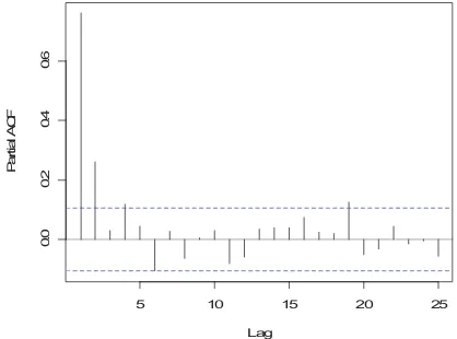
Figure 3. PACF of Opening Price Kedaung Indah Can Tbk Stock Before Differencing.
Based on Figure 1, it can be seen that the time series is not spread fairly stationary. Therefore, it
needs to do differencing. In addition, it is also examined the ACF and PACF to identify with certainty
the stationary property. Figure 2 shows autocorrelation of each lag hyperbolic decreased slowly
towards zero, while Figure 3 shows cut lag after lag p. This indicates stationarity and long memory
process, to solve this problem, the suited model which can be used is ARFIMA(p,d,q) model, where d
is long memory parameter.
3.3. Parameter Estimation
Differencing parameter d is estimated by using GPH method on opening price data from Kedaung
Indah Can Tbk stock, by developing macro on MATLAB 5.3 program, it is obtained a value of long
memory parameter d is 0.452.
Figure 4. Opening Price Data of Kedaung Indah Can Tbk Stock After Differencing. International Journal of Applied Mathematics and Statistics
0 5 10 15 20 25
0.
0
0.
2
0.
4
0.
6
0.
8
1.
0
Lag
AC
F
Figure 5. ACF of Opening Price Kedaung Indah Can Tbk Stock After Differencing d= 0.452.
5 10 15 20 25
-0.
1
0
-0.
05
0.
0
0
0.
05
0
.1
0
0
.1
5
Lag
P
a
rt
ia
l A
C
F
Figure 6. PACF of Opening Price Kedaung Indah Can Tbk Stock After Differencing d = 0.452.
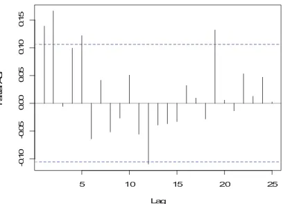
Plot the time series after differencing can be seen in Figure 4, in addition ACF and PACF plot after
differencing is presented in Figure 5 and Figure 6. Figure 5 shows that the lag q is cut at lag 1, 2, 4,
and 5, whereas in Figure 4.2.3 show that the lag p is cut at lag 1, 2, 5, 12, and 19. Therefore, there
are few estimates of ARFIMA(p,d,q) model to be tested. After going through the process of sorting
between the AIC, AICC, and BIC, ARFIMA model is obtained (5,0.452,4) as the best model with the
value of AIC = 3309.67, AICC = 3310.33, and BIC = 3348.07.
3.4. Diagnostic Checking
After obtained a model with significant parameters, it is necessary to do diagnostic tests including
checking residuals wheter they are independent and normally distribution or not. To examine the International Journal of Applied Mathematics and Statistics
independent of residual, it is used Ljung-Box test. The results of Ljung-Box test is obtained with
p-value = 0.9171tD for D= 0.05, this means that the ARFIMA(5,0.452,4) model has been qualified by
the independent of residual white noise. In addition to testing the residuals are independent, also
tested whether the residuals are normally distributed using the Kolmogorov Smirnov test. Results
obtained from the Kolmogorov Smirnov is a value of D = 0.054 and p-value = 0.2685tD. This means
that the residuals is normally distributed. Therefore ARFIMA(p,d,q) model which can be used at this
stage of the forecasting is ARFIMA(5,0.452,4) model.
3.5. Forecasting
On the opening price data from Kedaung Indah Can Tbk stock is obtained ARFIMA(5,0.452,4) as the
best model that can be used in forecasting. The model can be written as follows
t
t BZ
X
B) ( )
( 4
452 . 0
5 T
I
0.7863B 0.2094B2 0.2534B3 0.7113B4 0.1108B5)(1 B)0.452Xt
1 (
. ) 8494 . 0 4354 . 0 1572 . 0 7068 1
( 2 3 4
t Z B B
B
B
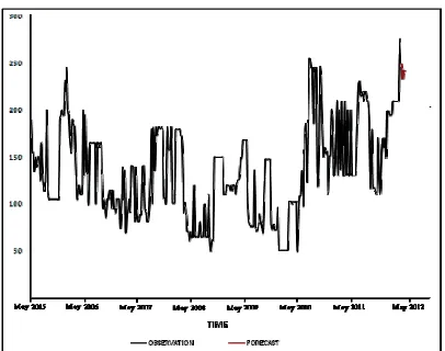
Table 1: Forecasting Result of Indah Can Tbk opening stock price.
Date Actual Forecast Se
02/04/2012 215 248.9972 29.56453
09/04/2012 245 248.7835 34.89799
16/04/2012 250 233.1545 39.15815
23/04/2012 255 241.9793 41.40609
30/04/2012 240 240.8529 41.14317
Index: se is square error.
Figure 7. Opening Price Data of Kedaung Indah Can Tbk Stock and Forecasting. International Journal of Applied Mathematics and Statistics
The forecasting results of ARFIMA(5,0.452,4) model for April 2012 are shown in Table 1 and Figure 7.
Table 1 is showing that result of forecasting for April 2012 having value which is close enough to its
actual data. This is to confirm ARFIMA model has given best suited for long memory process.
4. CONCLUSION
In this paper, it is studied forecasting long memory time series for stock price with model
autoregressive fractionally integrated moving average. This model is denoted by ARFIMA(p,d,q), that
is
, ) ( )
( t q t
d
p B X T BZ
I
where {Zt} is white noise, ( ) 1 1 ,
p p
p B IB I B
I " ( ) 1 1 ,
q q
q B TB T B
T " and d is the
fractional difference operator with d real number is located at 0d12. The model ARFIMA(p,d,q) is
applied to the opening price data of Kedaung Indah Can Tbk stock from May 2nd 2005 until March
26th 2012, the best suited model is ARFIMA (5,0.452,4). This model is good enough to forecast short
time prediction for long memory time series where forecasting result is very close to actual data with
small square error.
5. REFERENCES
Bisaglia. Model Selection for Long Memory Model. Quaderni di Statistica; 2002, Vol. 4.
Boutahar M and Khalfaoui R. Estimation of the Long Memory Parameter in Non-Stationary Models: A Simulation Study. GREQAM; 2011, version 1-23 May 2011.
Brockwell PJ and Davis RA. Time Series: Theory and Methods. Springer-Verlag. New York. 1991.
Granger WL and Joyeux R. An Introduction to Long Memory Time Series Models and Fractional Differencing. Journal of Time Series Analysis 1; 1980, 15-29.
Haslett J and Raftery AE. Space Time Modeling with Long Memory Dependence: Assessing Ireland's Wind Power Resource. Applied Statistics; 1989, Vol. 38, No.1, 1-50.
Hosking JRM. Fractional Differencing. Biometrika; 1981, Volume 68, 165-176.
Hurst HE. Long-Term Storage Capacity of Reservoirs. Trans. Am. Soc. Civil Eng.; 1951, 116:770-779.
Palma W. Long-Memory Time Series. John Wiley and Sons, Inc. New Jersey. 2007.
Wei WWS. Time Series Analysis. Addison Wisley Publishing Company. Canada. 1990. International Journal of Applied Mathematics and Statistics