PTR: Andy Shafran part of this book may be reproduced or transmitted in any form or by
any means, electronic or mechanical, including photocopying, record-ing, or by any information storage or retrieval system without written permission from Thomson Course Technology PTR, except for the inclusion of brief quotations in a review.
The Premier Press and Thomson Course Technology PTR logo and related trade dress are trademarks of Thomson Course Technology PTR and may not be used without written permission.
Maple 9.5 is a registered trademark of Maplesoft. All other trademarks are the property of their respective owners.
Important:Thomson Course Technology PTR cannot provide software support. Please contact the appropriate software manufacturer’s techni-cal support line or Web site for assistance.
Thomson Course Technology PTR and the author have attempted throughout this book to distinguish proprietary trademarks from descriptive terms by following the capitalization style used by the manufacturer.
Information contained in this book has been obtained by Thomson Course Technology PTR from sources believed to be reliable. However, because of the possibility of human or mechanical error by our sources, Thomson Course Technology PTR, or others, the Publisher does not guarantee the accuracy, adequacy, or completeness of any information and is not responsible for any errors or omissions or the results obtained from use of such information. Readers should be particularly aware of the fact that the Internet is an ever-changing entity. Some facts may have changed since this book went to press.
Educational facilities, companies, and organizations interested in multi-ple copies or licensing of this book should contact the publisher for quantity discount information. Training manuals, CD-ROMs, and por-tions of this book are also available individually or can be tailored for specific needs.
ISBN: 1-59200-038-X
Library of Congress Catalog Card Number: 2003105366 Printed in the United States of America
04 05 06 07 08 BH 10 9 8 7 6 5 4 3 2 1
Thomson Course Technology PTR, a division of Thomson Course Technology
S
o many people were involved in bringing this book to life, thanking each person individually would be a book in itself. Instead of subjecting you to that, I’ll break the deserving into groups. From the early-on mathematicians to the old-school demo programmer gurus who taught me the secrets of the PC, I thank you all for the invaluable technical knowledge. Special thanks to the University of Ottawa professors who could actually teach, a rarity in an educator (especially in the engineering field). Thanks to my personal stress relievers (that is, the Quake3knobs on XO server), which were like caffeine when the hours were late. Special thanks to everyone who shepherded this book through production; I think the end result speaks for itself. Finally, I would like to thank every sin-gle reader out there, without whom none of this would be possible. After you’ve mastered the material here, I call on you to create some kick-ass demo to make us all proud!CHRISTOPHERTREMBLAY lives in the California Bay Area, where he works for Motorola
building a 3D graphics engine for cell phones to power next-generation games. He holds a degree in Software Engineering from the University of Ottawa, Canada, and is currently completing final courses for a mathematics degree. His work in the game industry includes game AI, core-networking, software rendering algorithms, 3D geometry algo-rithms, and optimization. Although most of his work is PC-based, a fair amount of it was done on embedded devices ranging from bottom-line TI-calculators to Z80 and 68K Palm processors to speedy PocketPC strong-arm processors, with games such as LemmingZ.
About the Series Editor
ANDRÉLAMOTHE, CEO, Xtreme Games LLC, has been involved in the computing
indus-try for more than 25 years. He wrote his first game for the TRS-80 and has been hooked ever since! His experience includes 2D/3D graphics, AI research at NASA, compiler design, robotics, virtual reality, and telecommunications. His books are top sellers in the game programming genre, and his experience is echoed in the Thomson Course Technol-ogy PTR Game Developmentseries.
Introduction . . . xiii
Part I: The Basics
1
Chapter 1 Equation Manipulation and Representation. . . 3Choosing a Coordinate System . . . .4
Equation Representation . . . .14
Using Polynomial Roots to Solve Equations . . . .18
Substitution . . . .25
Chapter 2 Baby Steps: Introduction to Vectors . . . 29
O Vector, What Art Thou? . . . .29
Basic Operations and Properties . . . .31
Advanced Operations and Properties . . . .36
Vector Spaces . . . .45
Chapter 3 Meet the Matrices . . . 53
Meat, the Matrices . . . .54
Basic Operations and Properties . . . .55
Advanced Operations and Properties . . . .64
Matrix Decomposition . . . .81
Eigenvectors . . . .89
Diagonalization . . . .91
Vector Revision . . . .92
Chapter 4 Basic Geometric Elements . . . 95
Creating Lines . . . .96
Generating Planes . . . .98
Constructing Spheres . . . .101
When Elements Collide . . . .103
Know Your Distances . . . .115
3D File Formats . . . .123
Chapter 5 Transformations. . . 125
It’s All About the Viewpoint . . . .126
Linear Transformations . . . .128
Multiple Linear Transformations . . . .138
Projections . . . .144
Non-Linear Transformations . . . .151
Chapter 6 Moving to Hyperspace Vectors: Quaternions . . . 153
Complex Numbers . . . .154
Basic Quaternions . . . .158
Advanced Operations on Quaternions . . . .161
Part II: Physics
167
Chapter 7 Accelerated Vector Calculus for the Uninitiated . . . 169The Concept of Limits . . . .170
Derivatives (The Result of Differentiation) . . . .175
Reversing: Integration . . . .191
Chapter 8 Gravitating Around Basic Physics . . . 209
Move That Body... . . . .210
Physical Force . . . .215
Energy . . . .227
Chapter 9 Advanced Physics . . . 235
Oscillations . . . .242
Center of Mass . . . .257
Angular Forces . . . .259
Chapter 10 And Then It Hits You: You Need Collision Detection . . . . 263
Environmental Collisions . . . .264
Collisions of Objects Among Themselves . . . .269
Picking . . . .287
Part III: Playing with Numbers
293
Chapter 11 Educated Guessing with Statistics and Probability. . . 295Basic Statistics Principles . . . .296
Random Number Generation (Uniform Deviates) . . . .302
Distributions . . . .310
Intelligence Everywhere . . . .319
Chapter 12 Closing the Gap for Numerical Approximation. . . 323
Solution Approximation . . . .324
2D Function Approximation . . . .327
Multivariable Function Approximation . . . .358
Chapter 13 Exploring Curvy Bodies . . . 363
Splines . . . .363
Surfaces . . . .385
Part IV: Rendering and Lighting
389
Chapter 14 Graphics-Generation Engines . . . 391Decals . . . .392
Billboards . . . .397
Applications . . . .402
Chapter 15 Visibility Determination: The World of the Invisible . . . . 405
GPU-Level Visibility Determination . . . .406
CPU Culling . . . .409
Chapter 16 Space Partitioning: Cleaning Your Room . . . 427 Chapter 19 The Quick Mind: Computational Optimizations . . . 503
Fixed Points . . . .504
IEEE Floating Points . . . .517
Condition Arithmetic . . . .524
Chapter 21 Kicking the Turtle: Approximating Common and
Slow Functions . . . 563
Transcendental Function Evaluation . . . .564
Physical Model Approximation . . . .584
Appendixes
589
Appendix A Notation and Conventions . . . .591Trigonometric Definitions . . . .593
Appendix B Trigonometry . . . .593
Symmetry . . . .594
Pythagorean Identities . . . .597
Exponential Identities . . . .598
Cosine and Sine Laws . . . .600
Inverse Functions . . . .601
Appendix C Integral and Derivative Tables . . . .605
Appendix D What’s on the CD . . . .611
Sometimes it seemed like this day—the day that Mathematics for Game Developerswould be sent to press—would never come. Of the Game Developmentseries, this title has been one the most challenging books to develop. Not only was it difficult to decide just what the book should include, but finding the perfect author—one who was knowledgeable in both mathematics and game development and at the same time a fantastic writer—was virtually a statistical impossibility! After a lot of searching, however, I did find the perfect author: Christopher Tremblay. This book exceeds my expectations and I hope it exceeds yours.
Within Mathematics for Game Developers, not only will you find the entire landscape of relevant, practical mathematics laid out in such a way that you can understand, you will also see how it is connected to game programming. The book begins by covering vectors, matrices, and complex number theory, and then shows how those fields of study can be applied to real 3D problems. When this framework is in place, the book then covers physics modeling and collision detection, followed by approximations, statistics, and probability—which are especially important when you consider that 99 percent of all computer graphics are based on simplified models or approximations. The core of the book, on 3D graphics, includes coverage of such topics as 3D graphics algorithms, visibil-ity, rendering, and lighting techniques and their mathematical descriptions. Finally, the last chapters discuss mathematical optimizations as well as SIMD technology. (If you don’t know what that means, then you’d better read this book!)
In conclusion, there are a lot of game development math books out there, but none that are as accessible as this one, that give you as much practical information for real game development.
Sincerely,
André LaMothe
xiii
M
ath is a fundamental part of any game developer’s programming arsenal.With-out a strong understanding of math, you can easily waste days solving a prob-lem in a game that, in reality, is as simple as 1-2-3. If you’re considering programming a game that is even slightly complicated, you must realize that it is crucial to first master some basic concepts such as matrices and vectors.
This book is designed specifically for the game developer,notthe mathematician. Most game programmers interested in learning about the math behind their work have two options:
■ They can read a “true” math book—that is, a book that is geared for
mathemati-cians. The problem with reading this type of book is that they not only tend to delve so deeply into each equation, losing you in the process, but they also provide you with no means to understand the material.
■ They can read a “plug-and-play” book, which tend to present a glut of equations
without showing how everything fits together.
This book falls somewhere in the middle. It clarifies how mathematical ideas fit together and apply to game programming, and includes only those proofs that help elucidate use-ful math concepts. Unlike most math books—including many math books for game pro-grammers—this book is concerned less with whyit works (for example,provingthat one plus one equals two) as with howit works and what that implies.
n o t e
Unless otherwise stated, the logic and deduction found throughout the book will stand for real numbers. Sometimes it will stand for complex numbers or even the more general cases, but over-all, I won’t bother covering the more general cases.
Beyond teaching you the mathematical concepts you need as a game programmer, this book aims to teach you to think for yourself, outside the box. In many cases, the best-known method for solving a problem won’t be the simplest, fastest, or most efficient. Don’t be afraid to try an unconventional approach; it just might make a dramatic differ-ence in your game!
What You’ll Find in This Book
In this book, you will find some unique solutions for dealing with real problems you’ll likely face when programming many types of 3D games. Not only does this book show you how to solve these problem, it also explains why the solution works, which enables you to apply that solution to other problems that may crop up. Put another way, this book doesn’t just show you how to solve problems; it teaches you how to thinkin order to solve problems.
The main topics that this book tackles are
■ Fundamentals of mathematics
problems such as those seen in statistics for AI purposes, approximation for speedier functions, and interpolation for an ultra-smooth transition. Part IV, “Rendering and Lighting,” looks at the rendering pipeline and how things can be modeled in an efficient manner. It discusses methods for rendering a game world that not only looks true-to-life but also displays quickly and efficiently. The last part, “Optimizations,” takes a slightly less mathematical approach, discussing various techniques that can be used to optimize your code. It covers the use of fixed points for embedded devices, some dandy fast functions for basic math operations, and some crazy-fast approximations for well-known functions.
The Basics
Chapter 1
Equation Manipulation and Representation . . . .3
Chapter 2
Baby Steps: Introduction to Vectors . . . .29
Chapter 3
Meet the Matrices . . . .53
Chapter 4
Basic Geometric Elements . . . .95
Chapter 5
Transformations . . . .125
Chapter 6
Moving to Hyperspace Vectors: Quaternions . . . .153
3
Equation Manipulation
and Representation
C
ontrary to popular belief, mathematics is not a universal language. Rather, mathe-matics is based on a strict set of definitions and rules that have been instated and to which meaning has been given. Indeed, arguably, logic is simply the process of someone else making you believe that what you know truly makes sense. In reality, a state-ment such as “1 + 1 = 2” is as “logical” as the statestate-ment that a chair is “a chair as we know it.”Likewise, mathematics for game programming, which is primarily an algebraic field, is also based on a set of definitions and rules. I assume that you already have reasonable knowledge of these algebraic rules; this chapter is meant to both refresh your algebraic knowledge and, perhaps, extend it a bit. That said, I hope that in addition to teaching you how to apply this set of definitions and rules to game programming, this book will open your mind to new ways of thinking about and representing problems. This chapter assumes that you know trigonometry and that you have taken a look at Appendix A, “Notation and Conventions,” which enumerates a few interesting identities and refreshes your memory with regards to the relationships between trigonometric functions and a unit circle.
This chapter covers the following:
■ Choosing a coordinate system ■ Equation representation
Choosing a Coordinate System
One important thing to consider when writing a game is the coordinate system you choose to use. As you’ll discover, every coordinate system has its own purpose; that is, each one is geared toward performing certain tasks (this will become evident as I enumerate a few of them). So, although an infinite number of coordinate systems exists, a few stand out for writing games:
But wait, what exactly is a coordinate? You can define a coordinate as being a set ofn vari-ables that allows you to fix a geometric object. You should already be familiar with coor-dinates and also a few of these systems, but chances are that some of them will be new to you. Admittedly, not all of them are terribly useful for game programming, but I added them to expose you to a new spatial system, a new way of thinking.
n o t e
All coordinates will be presented in a vector form <a, b, c, . . . > with length smaller or equal to n corresponding to the space’s dimension.
Cartesian Coordinates
Without a doubt, the Cartesian coordinate system is the most widely known coordinate system. As shown in Figure 1.1, the Cartesian coordinate system is a rectilinear coordinate system—that is, a system that is rectangular in nature and thereby possesses what I will call rectangular coordinates. Each component in the Cartesian coordinate system is orthogonal. Geometrically speaking, this implies that each axis of the space is perpendic-ular (90º) to the other axis. Because of its rectangperpendic-ular nature, this system can naturally do translations by mere addition.
is [⫺⬁,⬁]. For the sake of example, I’ve plotted <1, 2, 3> on a 3D Cartesian system (feel free to do the same); the results are shown in Figure 1.2.
Figure 1.1
A 2D Cartesian coordinate system
Figure 1.2
Interestingly enough, this by no means implies that the Cartesian coordinate system you use should be such that xis horizontal,yis vertical, and so on. You could easily build a Cartesian coordinate system where, for example, the zandyaxes are inverted. Just make sure to take this into account when plotting the coordinate. Similarly, you can define which side of the axis is negative and which one is positive, also called handedness, as illus-trated in Figure 1.3. Typically, this only involves a change of sign in the depth axis, and this line is usually only drawn from the origin to the positive side of the axis, thus generating what looks like a house corner from the perspective of the inside or outside. For example, in 2D, using a 2D rendering library, the screen is arranged such that the yaxis diminishes when moving up, but the xaxis stays the same. This implies that the origin is at the top-left corner of the screen, instead of being at the bottom-top-left like a Cartesian coordinate system would yield. Math books sometimes like to place the 3D yaxis as the depth com-ponent and the zaxis as the height, but here I will stick to what the 3D libraries use.
t i p
In Maple, you can use the plot([<functions(x)>], x=a..b, <options>) or plot3d([<functions>(x, y)], x=a..b, y=c..d) to plot graphs using Cartesian coordinates.
Polar Coordinates
Thanks to trigonometric primitives, the polar coordinate system is probably the second best-known coordinate system. As shown in Figure 1.4, the polar coordinate system is a radial coordinate system—that is, a system that is characterized by its distance relative to Figure 1.3
the center of the coordinate system. The polar coordinate system is a 2D coordinate sys-tem, and has the property of being cyclic in one component. It possesses two components: <r,>.ris the radial component, and it specifies the distance from the origin;is the angular coordinate, and represents the angle from an arbitrarily defined starting point.
Because of its circular nature, the polar coordinate system is very well adapted to rota-tions, which are performed naturally with an addition to the angular component. The range for this coordinate system is <[0, 2), [0,⬁]>.
You can easily convert from polar coordinates to Cartesian coordinates with the following relationship:
Conversely, you can convert from Cartesian coordinates to polar coordinates with the fol-lowing relationship:
Figure 1.4
Let’s plot <1, 2> on a polar coordinate system; Figure 1.5 shows the results.
t i p
In Maple, you can append the coords=polar option to the plot function in order to plot graphs using polar coordinates.
Bipolar Coordinates
In a polar coordinate system, all coordinates are described with an angle and a length. A bipolar system, on the other hand, is described with two lengths or two angles. Although the bipolar coordinate system is not a very popular coordinate system for gaming pur-poses, it does have its uses and makes for a great way to look at things differently. Just as its name suggests, a bipolar coordinate system is minimally equipped with two centers, the distance between which can be a. For mathematical simplicity, let a= 2c.
Consider only the bipolar coordinate system, which is described with two lengths,r1and
r2,as illustrated in Figure 1.6. It may be a little confusing to see how you can pinpoint a
coordinate with two lengths, but it is actually quite simple. The coordinate described by <r1,r2> is the point at which the two circles of radiusr1andr2, separated by a,intersect. As illustrated in Figure 1.6, for any two circles, there should be two intersections (assum-ing there is an intersection at all). As with the polar coordinate system, the range of the lengths is [0,⬁].
Figure 1.5
You can convert from bipolar coordinates to Cartesian coordinates with the following relationship:
Conversely, you can convert from bipolar coordinates to Cartesian coordinates with the following relationship:
Figure 1.6
One good use of this system is illustrated by the equation of an ellipse. An ellipse can eas-ily be expressed in bipolar coordinates with its well-known relationship between its foci, r1+ r2=2a, as illustrated in Figure 1.7.
Now that you have the basic idea, think a bit more about the new material and see what else you can come up with. The bipolar coordinate system shown here is cumbersome because it does not uniquely determine a single point in space. Try applying the same idea of intersection using angles instead. You will notice that they can uniquely determine a coordinate. You can also start to think about how this general idea can be applied to 3D to generate funky objects such as ellipsoids or smooth spherical-like objects. At this point, the stage is yours.
t i p
In Maple, you can append the coords=bipolar option to the plot function in order to plot graphs using bipolar coordinates.
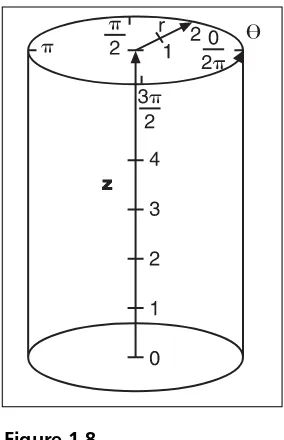
Cylindrical Coordinates
One rather interesting coordinate system for 3D coordinates is the cylindrical coordinate system, shown in Figure 1.8. This system mixes the polar coordinates with the Cartesian coordinates to get the best of both worlds when a mixture of both is required. As the name suggests, cylindrical coordinates are contained in the form of a cylinder, which is defined by three parameters: <r,,z>. The first two parameters are associated with the polar space Figure 1.7
and have the same interpretation. The z component is associated with the Cartesian z coordinate, and also has the same purpose. This set of coordinates can be very useful when a rotation around one single axis is required, as well as when translations along the axis are required.
The ranges for the parameters are also the same as their two respective coordinate systems: <[0, 2), [0,⬁], [⫺⬁,⬁]>. Converting from cylindrical to Cartesian is easily done with the same relationships established earlier:
From Cartesian to cylindrical, the conversion is as follows: Figure 1.8
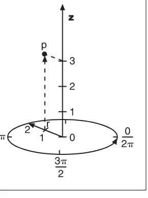
If you wanted to plot <1, 2, 3> on such a system, the results would be as shown in Figure 1.9.
t i p
In Maple, you can append the coords=cylindrical option to the plot3d function in order to plot graphs using cylindrical coor-dinates.
Spherical Coordinates
The next obvious progression from Cartesian to cylindrical is the spheri-cal coordinate system illustrated in Figure 1.10. Whereas the cylindrical coordinates introduced an extra rec-tangular dimension to the polar coor-dinates to take care of the depth (or height, depending on your angle), the spherical coordinates introduce an extra component to the polar nates to uniquely access all coordi-nates in 3D. That being said, the spherical coordinates have three para-meters: <r,,>.
Figure 1.9
A coordinate plotted using cylindrical coordinates
Figure 1.10
This system can naturally do rotations around any two axes in 3D space with a mere addi-tion. The range of the parameters is <[0,⬁], [0, 2], [0,]>. Notice that the second angle is not bound to 2, which makes sense because if you were to allow it to comprise values greater than , you would be in a situation where the coordinate would not be uniquely defined by the three parameters, and hence the redundancy would not be necessary.
By carefully looking at the geometry of the problem, and with some help from trigonom-etry, you can deduce that the conversion from spherical coordinates to Cartesian coordi-nates can be obtained with the following:
Conversely, you can convert from Cartesian to spherical coordinates with the following equation:
Once more, if you stand by your sample coordinate <1, 2, 3>, you obtain the plot in 3D space, as shown in Figure 1.11.
Figure 1.11
t i p
In Maple, you can append the coords=spherical option to the plot3d function in order to plot graphs using spherical coordinates.
Equation Representation
An equation is a formal statement of equality between two mathematical expressions. For example, a statement like x=a+ 1 is an equation because it is composed of an equality between the expression xanda+ 1. Equations can be represented in a few ways. This book focuses on three types of equations, each with its own pros and cons. As you will see, some representations are very well adapted to certain uses and, as with the various coordinate systems, each equation representation has its own way of “naturally” dealing with certain types of problems. In this section, you’ll learn about the three types of equations on which this book focuses, and you’ll see how to convert from one system to another (whenever possible). Understanding how to solve equations is a key and basic concept that will serve you throughout this book.
Do You Function Correctly?
By far the most widely known way to represent an equation is via a function. A function can be sloppily defined as a relationship for which every set of input maps to one single value. Generally speaking, you have a function if one side of the equation has only one variable. When this is the case, the input parameters of the function are the variables on the opposite side of the equation.
A function is typically written as f(x,y,z), where x,y,zare the parameters of the function. For example,f(x) =2x + 1is an example of a function; more precisely, it is the equation of a line. Geometrically speaking, with a 2D function’s graph plotted in a Cartesian coor-dinate in which xrepresents the horizontal axis, any given vertical line of infinite length should intersect with the graph no more than one time. This is also true for the general case. If you think in 3D, a very similar deduction can be put forward using a plane and a 3D graph. Once more, this is true because we claimed that ashould have no more than one value per input set.
t i p
In Maple, you can assign values to variables via the assignment operator :=. Similarly, you can also define functions with this method. You may also unassign an operator with the command unassign(‘operator’).
Parametric Notation
This equation description format is much less restrictive than a function because it does not force any variable to have only one value per input set. It enables you to freely describe the equation by giving one function for every coordinate in the coordinate system. Although these equations permit more liberal movement in space, some are somewhat cumbersome to deal with because they have more than one value per input set. Because these equations do not yield a unique value per input set, they obviously cannot be con-verted from a parametric form to a functional form. The following examples are equa-tions in parametric form:
Figure 1.12
Graph of a square root
Figure 1.13
Converting a function to parametric notation is actually quite easy: Simply leave all the input parameters as is, and make the result of the function the last parameter. It does not come easier than this. Take the following as an example:
The challenge is when you want to convert from parametric to functional. The trick here is to isolate the parameters and substitute them into the other equations. In some cases, you can get a single equation by substituting every parameter, but you may sometimes end up in situations where you can no longer substitute. This is not always a problem; it sim-ply implies that one of the variables is not really important in relation to the variable you have isolated for. Clearly, you may lose some information by doing this, but it will convert the equation to a function as required. For example, take the following equation of a plane in 3D:
There is no easy conversion trick for very complicated equations. The best thing you can do is look at your function geometrically (if possible) to see whether it has only one value per axis. To make this possible, you might want to consider changing your coordinate sys-tem with the substitutions mentioned earlier in this section. The circle is obviously not a function because it has two values for any vertical or horizontal line, but if you change to polar coordinates, you can convert everything into a function, as shown here:
t i p
Maple also accepts parametric input for equations using plots by issuing brackets around the func-tion and defining each input set plus the range of the input parameters. To do so, issue the com-mand Plot([fx(s), fy(s), s=a..b]); for 3D plots, the comcom-mand is plot3d([fx(s, t), fy(s, t), fz(s, t)], s=a..b, t=c..d).
Figure 1.14
Chaotic Equations
The last types of equations are neither parametric nor functional—although they may look functional at first. The problem is, it is impossible to isolate one of their variables. For example, try to isolate any of the variables in (8+2x + x2= y2⫺y) to yield a function; you
will quickly discover that it is not possible. In general, these equations are not easy to con-vert into another representation—indeed, doing so is sometimes impossible algebraically.
This book doesn’t focus much on these types of equations, but you will look at a few things about them in the chapters to come. Converting them from their original form to parametric or functional form requires various tactics and techniques. At the very least, you’ll explore one method that, in fact, can solve the problem in the preceding paragraph and a family of similar problems.
Using Polynomial Roots to Solve Equations
Polynomials are equations of the form y = anxn+ … aixi+ a0x0. This section focuses on
finding the roots of a polynomial—in other words, solving algebraically for xin the equa-tion 0= anxn+ … aixi+ a0. As you will soon see, there is more to this than simply finding
a finite set of solutions for x.
Quadratic Equations
Quadratic equations are second-order polynomial equations—in other words, equations of the form ax2+ bx + c= 0, where {a,b,c} are constants and xis a variable with a power
of at most two (hence the word second). What’s interesting with these equations is that you can easily determine the values for x. Specifically,xhas two values, but they are not guar-anteed to be real. The trick to isolating xcomes from a process called “completing the square.” (This process can also be useful when dealing with other problems.) The idea is to express the equation as a square ofxplus some value. The benefit of doing so is that you can then determine the square root on each side to end up with one single value ofx.
You are probably familiar with the following general root-finding quadratic equation:
The square is completed on the fourth line, where two canceling terms are added and one is pulled out of the parentheses so that the resulting equation can easily be converted to the square of some value, thereby reducing the power ofx. This equation is really inter-esting because it is very similar to the previous one. Its bottom portion is exactly the same as the first one’s top portion. This gives the interesting identity, which can yield more sta-ble floating-point values for two different roots:
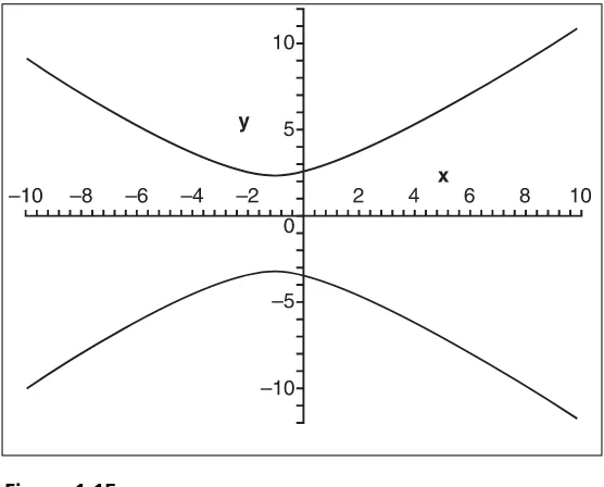
Now that you have two solutions for a quadratic equation, you can actually do something with the equation 8+2x + x2 = y2⫺y, illustrated in Figure 1.15.As long as one of the
Isolating for yyields a slightly nicer result, so let’s proceed:
This is obviously not a function because it always has two values for any value ofy. This equation is, however, a piecewise function, which means that by breaking this equation into pieces (in this case, two), you can construct well-defined functions. Obviously, by handling the plus/minus cases separately, you can do this. Later on, you will see how you can convert this equation into a pure function in certain conditions. Because the square root is defined only in real space for positive values, the discriminant, which is an expres-sion distinguishing between two entities (here,b2⫺4ac), must be greater than or equal to
Figure 1.15
0 for the solutions to be real. If the discriminant is 0, then two real solutions, which are exactly the same, exist. This is obvious because the square root of 0 is 0, and that 0 is not affected by a negative or positive sign.
Cubic Equation
If you managed to find a solution for a quadratic equation, one cannot help but think that a similar process can be performed to find a solution for a cubic equation. Sure enough, it is possible. The proof of this derivation is rather tedious, so I will skip it. Most of it is done by a set of variable substitutions, which you will see clearer examples of shortly, and by completing the cube.
A cubic equation is a polynomial of the form x3+ ax2+ bx + c=0where {a,b,c} are con-stants and xis a variable. To calculate the solution of such an equation, you must compute things in a few steps, which mainly come from the substitutions the proof/derivation requires. You must first compute two values:
Once you have these two values, you need to verify that R2<Q3. If so, then the following holds:
The solution is then given by the following:
Notice how only one real root exists in this scenario. In order to illustrate how this works, take the equation x3+5x2⫺22x + 16.
x= {-8, 1, 2}, which makes perfect sense if you verify by reversing the process and multi-plying (x + 8)(x⫺1)(x⫺2). If you look at the curve this generates, you can see why I
went with this algorithm. If the curve was such that it was only intersecting at one loca-tion, this is where you would have to resort to the second path.
Quartic Equation
As with quadratic and cubic equations, you can find a solution to a quartic equation by applying a set of substitutions and clever algebraic tricks to reduce the terms. The deriva-tion can also make use of the Viéta formula, discussed in Chapter 11, “Educated Guessing with Statistics and Probability,” or substitution combined with two passes to complete the square.
A quartic equation is the next logical step after the cubic polynomial equation. That being said, a quartic equation is of the form x4+ ax3+ bx2+ cx + d= 0, where {a,b,c,d} are constants and xis a variable. Due to the increasing complexity of the derivations, I have broken the solutions into finite steps. Let’s start with a few precalculations:
The next step is to solve a cubic equation by finding two of its non-zero real roots:
Then, the four roots of the quartic equation are defined by the following:
Partial solutions for quintic equations also exist, but there is no known general solution for quintic equations. Generally, the trick to determining whether it’s possible to find a solution for a given partially polynomial equation is always pretty much the same: Try to factor the equation in a binomial equation (ax + b)nthat is a perfect power. When you
have this, you can take the nthsquare root and xwill be isolated. In order to get the equa-tion on one side into this format, you will need to do a few substituequa-tions, which is exact-ly what I’ll talk about next.
t i p
Maple can solve equations algebraically when a solution exists with the function solve(<function>, <variable>).
Substitution
Substitution is a very powerful tool that can be used to solve certain types of equations. You used substitution to some degree when learning about the various coordinate systems, but I think it’s appropriate to take a more complete look at the methods and tricks you can use to simplify your equations—or even obtain a well-defined formula for equations that did not initially have one.
Now you want the first-order term to be 0, which implies the following:
Geometrically speaking, the substitution applied is a horizontal translation of three quar-ters to the right. We did not actually change the function at all at this point because the equation is in terms ofyand not in terms ofx. If you want the equation to be a function ofx, then you have to apply the reverse process:y=x⫺a. So for example, if you wanted to know the value off(x) for x= 4, you would have to compute f(4 + _) for f(y), which gives 39, the same answer as f(x) for x= 4. This method is particularly interesting for com-putational complexity because it successfully reduces a multiplication to a simple sub-traction.
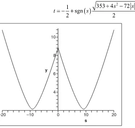
Substitution also enables you to convert an ugly equation into a function or parametric form with a rather interesting trick. Using this chapter’s earlier example of a quadratic equation, suppose that you are interested only in the range ofx= [⫺10, 10] for that equa-tion. By applying a substitution, you can make it such that the equation takes only posi-tive values as input. Then, you can take advantage of this equation’s symmetry in order to take care of both cases in the same equation. If you can achieve this, you will successfully convert the equation into a function. Observe the following logic:
Let’s perform the substitution x=s⫺10. This also changes the domain for xto [⫺10 +
In this equation,sis always expected to be greater than 0, so you can substitute sfor the absolute value ofswithout changing anything. Also note that s2is always positive regard-less of the sign ofs. The trick to solve this one stems from the fact that you can store infor-mation using the sign ofsby allowing it to span from [⫺20, 20] and by adding extra logic in the equation to change the sign whenever sis negative. Observe the following change in the equation and its resulting graph (see Figure 1.16):
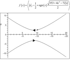
This does not solve the problem entirely; it simply generates another similar mirrored curve in the negative xquadrant. This is to be expected, though, because you know that a function can have only one value for any input, while the parametric notation does not have this limitation. The final trick to solve this as a parametric equation is simply to notice that sshould always be positive, regardless of what happens. This last fact gives the following equation and graph (see Figure 1.17), which is exactly like the chapter’s first equation, but translated by 10—which means that a substitution ofs=x+ 10 can convert your values for xinto well-defined values for s.
Figure 1.16
If you distinguish the difference between +0 and ⫺0 like the floating-point IEEE format does, this is a fully valid equation. If you cannot distinguish between these two, then you have a problem because 0 has no sign defined and, as a result, the equation is not defined.
t i p
Maple can also perform substitutions via the evaluation function eval(<equation>, <var> = <func-tion or value>). Sometimes, the equa<func-tions Maple yields are not simplified, so simplify(<equa<func-tion>) may come in handy. Another very useful tool is the expand(<equation>) function, which can break up the function powers and effectively undo some level of simplification.
Figure 1.17
29
Baby Steps: Introduction
to Vectors
You probably already know a good deal about vectors. In fact, you may be considering skipping this chapter altogether. My advice: Don’t. This chapter will serve as a good review and reference for more advanced topics you will tackle later on. Along the way, you may also find some new and interesting ways of seeing things, which may open your eyes to some relationships between certain elements. I have also placed a few Easter eggs in this chapter if you think you know all there is to know about vectors.
n o t e
Vectors are a very abstract concept and can be applied to many things. This book is interested in vectors primarily with regard to how they relate to real numbers; for this reason, some definitions and relations you’ll find here work for real numbers only.
This chapter covers the following:
■ Defining vectors
■ Advanced vector operations and properties ■ Vector spaces
O Vector, What Art Thou?
that a coordinate is a vector, but not quite directly. A vector has a direction and a magni-tude, and does not have a fixed position in space. You could claim that a coordinate is a vector from the origin (more on this later). Because of this, and for practical reasons, this book will use the vectorial notation for coordinates (which is identified by a bold charac-ter). For example, suppose you wanted to assign a direction to a point in space. In that case, you would require two things: one coordinate and one vector.
n o t e
Although vectors are not like coordinates per se, they are fairly similar to polar coordinates because both are described with a magnitude (length) and a direction (angle).
Another way to see a vector is to look at it as an offset coordinate, as was initially men-tioned, with the stretched definition of a coordinate as being a vector from the origin. A vector is defined by ncoordinates, where each component is typically assigned one axis in the coordinate system. You can also call these n-vectors. Most applications that use vectors use 2-vectors and 3-vectors.
Vectors are commonly expressed in a Cartesian coordinate system <x,y,z, . . . >, but you can use the same principles in another coordinate system, such as in Polar coordinates, for example <,r>. In fact, you can define a vector in any coordinate system. To do this, you use the concept of head and tail. A vector starts from its tail and ends at its head, as illus-trated in Figure 2.1. In Cartesian coordinates, a vector is typically expressed as two coor-dinates in space—for example,aandb. The vector ab(that is, the vector between a and b in that very order), starts at a(the tail) and ends at b( the head). Thus, a coordinate pin a coordinate system can actually be viewed as the vector 0p, where 0is the origin.
To compute the value of the vector, you would use the following: Figure 2.1
Likewise, if you have a coordinate aand a vector v, you can find your second coordinate bby simply inverting the process:
n o t e
The vector abin the preceding equation is not to be confused with a times b. Throughout this book,
I shall explicitly express the multiplication with a dot when confusion could arise.
It may sound confusing at first, but vectors use their own coordinate system, called a vec-tor space, which is relative rather than absolute. For example, if you expand the first equa-tion into components for the polar coordinate system, you get the following:
Geometrically, a vector can be seen as an arrow. The arrow indicates the direction, and therefore enables you to differentiate the tail and the head as shown in Figure 2.1. Because vectors do not actually possess an origin, the tail can be placed anywhere in coordinate space. The only restriction is that the head must lie at a given distance from the tail. For example, a vector <1, 2, 3>, which is written similarly to a coordinate, means that the tail is separated from the head by the signed numbers <x= 1,y= 2,z= 3>.
t i p
In Maple, you can define a vector by using triangular brackets, where the components are delim-ited by spaces. For example, a vector s= <1, 2, 3> would be defined as s= <1 2 3>.
Basic Operations and Properties
Direction Inversion
A vector has a direction; that’s a given. But how do you invert the direction of the vector? If you think about the problem geometrically, it is very simple. The head becomes the tail and the tail becomes the head. For example, suppose vector ab is defined and you want to determine the inverse of that vector. To do so, you simply swap a and b, and you get ba. It’s as simple as that.
If you think of vectors in terms of Cartesian coordinates, inverting the vector is a simple matter of swapping the two coordinates—which, as it turns out, is the exact same thing as multiplying everything by ⫺1. So in short, inverting the direction of a vector is pretty
sim-ple. You can simply multiply each of its coordinates by ⫺1, and voilà.
Hi! My Name Is Norm
As mentioned previously, a vector is defined as having a magnitude and a direction. You already looked at various aspects of a vector’s direction, but you haven’t yet explored the issue of magnitude, also called norm.
The norm of a vector, which can be represented with either single bars or double bars, is defined as follows:
It may come as a surprise that although this equation is generally accepted as the defini-tion of the norm of a vector, it is, in fact, only partially accurate. In truth, a norm in the general sense is defined as a function that attributes a length, size, or extent to the object being studied. It is not bound to one specific formula. The commonly used vector-norm, as stated in the preceding equation, fits just one group of norms called the p-norms. More specifically, it is defined as the 2-norm. The p-norm defined for pgreater or equal to 1 is as follows:
One thing that might have attracted your attention in Table 2.1 is the infinity (⬁) norm. The⬁norm is defined as the maximum absolute value of one component. If you look at the norms for increasing values ofp, you can see that the value converges toward 3. This book has not yet covered convergence, so I won’t go into it here, but keep your eyes open for Chapter 7, “Accelerated Vector Calculus for the Uninitiated.”
To see the graphical representation of what various values of the p-norm do to an input value in 2D, take a look at Figure 2.2, which illustrates various values ofp.
t i p
In Maple, you can compute p-norms by issuing the norm command with the vector as well as p, like so: norm(s,p).
A lot has been said here about thep-norm, but by all means, it is not the only norm you can use. For a norm to be at all use-ful, you need it to follow a fixed set of rules, which are defined as follows:
Table 2.1
p-Norm Values for
s
= <1,
⫺
2, 3>
p Expression p-Norm Value
1 6
2 3.7416. . .
5 3.0052. . .
⬁ 3
Figure 2.2
Given these rules, you can come up with your own norm if you do not like the generally accepted 2-norm. The logic still stands. That said, nicer results can be obtained with the 2-norm simply because of its circular nature. For this reason, the rest of the book assumes the use of a 2-norm.
Before you move on, there is one more norm-related concept that you need to grasp: You can say that an element is normal if it is of norm 1. If the element is not normal, then you can normalize the vector by dividing by its norm. For example, if you wanted to normal-ize <1,⫺2, 3>, you would apply the following logic for the 2-norm:
Thus, as soon as you need something related to the distance, the choice of norm truly is yours. Nothing really says that the 3-norm is better than all the other ones. The 2-norm is nice due to its circular nature, but the 1-norm and infinity norm can be equally useful— for example, in collision detection.
Vector Addition
If you compute everything step by step, you get the following:
Addition on vectors is defined such that you simply need to add every like component together. Thus, given vectors sandt, you can define their addition by the following equa-tion:
Similarly, you can define their subtraction by simply inverting the second vector, hence multiplying all its components by ⫺1. If you do this, you will quickly notice that given the addition rule, you can define the subtraction rule as follows:
Figure 2.3
When you want to add vectors using their coordinates, you can simplify the expression as shown above. You can replace these two vectors by the more direct vector generated by the tail of the first one and the head of the second, as shown previously in Figure 2.2. If you think of vectors as offsets, you can clearly see that adding two offsets is really the same as expressing this as one offset (which is really the sum of the two initial offsets). For exam-ple, if Mike walks for two miles and then turns around and walks for one mile, he is one mile from his initial position. As a more complex example, consider if you were to take the summation of a set of vectors. You may be able to simplify them as follows:
Algebraically, vectors can be manipulated using many of the laws you take for granted with real numbers. Most notably, the following can be used:
t i p
In Maple, vector addition can be performed in the exact same way you would add any other ele-ment type (for example,s+t).
Advanced Operations and Properties
When I talk about advanced operations, “advanced” is a relative term. Advanced opera-tions are just operaopera-tions that are more complex than basic elementary math. Mathematicians have defined most of these operations by forcing them to abide by a given set of rules and by then proving various results given the rule set. This is very similar to what you saw with the norm, where the norm is generally defined with a set of rules and where you can define, if you wish, more specific cases of the general set.
Dot Product
Wrongfully, the dot product is sometimes called the inner product. Although this is par-tially correct, in that the dot product belongs to that family, it is not precise to say so. The dot product yields its name from its notation. Given two n-dimensional vectors sandt, the dot product is defined as follows:
Note that this is not the same as the dot you use while programming. In programming, the dot is a period; in this case, however, the dot is centered with the characters. Multiplication on variables is implicit, meaning that when the variables are connected as in the preceding equation, a multiplication is implied. You may sometimes, however, have to resort to using variables with more than one character, which yields confusion about the variables’ names. It is therefore convenient to separate them with a dot, which is why you sometimes see equations written such that a dot separates two real variables that need to be multiplied. This is also sometimes applied to functions or multiplication between other types of elements. The dot product is actually the implied symbol in these cases because if you look at the function for n= 1, you will notice that the operation defines a simple multiplication.
By itself, the dot product is not interesting. What makes it interesting is an equation that the dot product satisfies. Notably, for two vectors sandt, and theta, the angle between the two vectors, you get the following:
t i p
In Maple, the dot product between two vectors sand tcan be computed with a period like so: s.t.
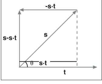
The geometrical interpretation comes from the equation. Take the previous equation and divide each side by the product of the norms. What you get is that the dot product of two normal vectors equals the cosine of the angle between them. Figure 2.4 illustrates what this means geometrically when sandtare normal. The result of the normal dot product is called a projection—in this case, an imaginary line that goes froms’s head to tby hitting tsuch that the imaginary line and tare perpendicular (that is, separated by an angle of 90 degrees). There is no real reason to normalize s; as long as tis normalized, the projection still works out perfectly. Therefore, if you look at the dot product where only tis normal, what you get is the projection of s upon the unit vector t.
You can easily see in Figure 2.4 that if you extend ssuch that it goes outside the unit cir-cle, you can still apply a proper projection ofsupont. This still follows the definition of cosine, as shown by the following equations:
Figure 2.4
Unfortunately, this does not work ift’s norm is not 1.
You can deduce a few more things from the dot product given its geometrical interpreta-tion and equainterpreta-tion:
■ If two vectors are perpendicular, geometrically, you can see that the result of the
dot product should be 0 because the projection of the first vector upon the second one is 0.
■ The dot product is in fact a good test for determining whether two vectors are
orthogonal. (Orthogonal is another way of saying perpendicular, but without the geometrical undertones.) As usual, do not restrict yourself to a mere 3D world. This definition is valid for an n-vector, so it can determine orthogonality for a 4D world if you can visualize such a thing. (If you figure out how, e-mail me!)
■ You can quickly determine whether two vectors are separated by less than 90
degrees by simply looking at the sign of the dot product. When the sign is positive, it means that the two vectors are separated by less than 90 degrees. (You can verify this by taking two normal vectors and substituting theta with a value of less than 90 degrees.)
One more thing of note: This function gives some form of “length” to a pair of vectors. This sounds an awful lot like a norm, except that this function allows for negative lengths and two vectors. To fix this, you can take the dot product of the vector upon the vector itself and it will always yield a value greater than 0 given a non-zero vector. Interestingly enough, if you do this, you will quickly realize that the square root of the dot product is in fact the 2-norm, as shown here:
Projection of a Vector Upon a Vector
Because you are projecting a vector upon another vector, you should logically get back a vector. If you look back at Figure 2.4, you will notice that the projected length is actually along the vector t. This makes sense because if you are projecting sont, then your vector should be a multiple oft. In order to compute the vectorial projection of a vector upon another, you simply need to change t’s length from whatever it may be to the projection length determined in the preceding equation. Simply put, start by normalizing the vector, thus giving it a length of 1 followed by a multiplication of the desired projection length, which you computed above. This yields the final equation for a projection ofsont:
As an example, take the same values chosen above for sandt. The projection ofsupont is computed as such:
Cross Product
The cross product, sometimes called the vector product, is another very important func-tion to master. It is defined only for 3D vectors, but you could also use it in 2D with 3D vectors by simply setting the last component of the 3D vector to 0. The cross product is represented with a cross. Its equation operating on two vectors,sandt, is as follows:
This is in fact one of the most cumbersome ways to remember the equation; in Chapter 3, “Meet the Matrices,” you will revisit the cross product by looking at it from a different angle. In that chapter, you’ll see equations that make its computation much easier to remember.
If you recall what it means to have the dot product of two vectors equal to 0, you proba-bly also recall that it implies that the two vectors are in fact perpendicular to each other. Thus, the cross product ofsandtcan geometrically be seen as a function that generates a vector orthogonal to both sandt. Another way to have the dot product yield 0 is if one of the two vectors is 0. What does it mean for the cross product ofsandtto be 0? The trivial solution is where sandt are 0, but this is not really interesting. Alternatively, ifs andt are linearly dependent (that is, parallel), the result of the cross product will be 0. This should come as no surprise because if you think about the geometrical implications, given two parallel vectors, you can generate an infinite number of perpendicular vectors, as shown in Figure 2.5.
So far, every operation you have seen could be handled using the same basic laws you are accustomed to using with real numbers. This, however, is where it all ends. Specifically, the cross product is not commutative. That means s•tis not the same as t•s. (You can easi-ly verify this by expanding the equation on each side.) Thus, the cross product can yield two perpendicular vectors.
If you think about the geometrical implications of this, it makes sense because you can select a vector and invert its direction to yield a new vector, which is also perpendicular to Figure 2.5
the other two and parallel to the previous. This is somewhat problematic, however, because you do not know which direction the new vector will go when you compute this.
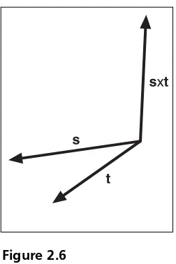
A very simple way to determine the new vector’s direction is to use the right hand rule. First, open your right hand and let your thumb make a 90-degree angle with your fingers. Next, point your fingers at the first vector of the cross product. Then, if possible, curl your fingers such that they point in the direction of the second vector. If you can curl your fin-gers in this way, then the resulting vector will be dictated by your thumb’s position. If you cannot curl your fingers because doing so would require you to bend them backward, rotate your hand such that your thumb points downwards. This should enable you to curl your fingers in the right direction, thus implying that the resulting vector would be point-ing downwards.
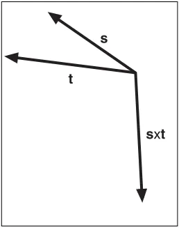
The right hand rule is a visual technique to determine the direction of the resulting vec-tor, but there is also a geometrical way to look at the problem. If going from sto trequires you to move in a counterclockwise fashion, then the vector points upwards. If the motion is clockwise, you are looking at a downward vector. Trigonometry offers yet another view of the problem. If the angle between sandt is smaller than rad, the vector will point upwards. If not, it will point downwards. Here, when the angle is computed, you should be looking at an angle range that increases in a counterclockwise fashion. Do not simply take the smaller of the two angles between the vectors. Figures 2.6 and 2.7 illustrate the concept.
Figure 2.6
Taking back our traditional values s= <1,⫺2, 3> and t= <0 ⫺1, 2>, you can compute their cross product as follows:
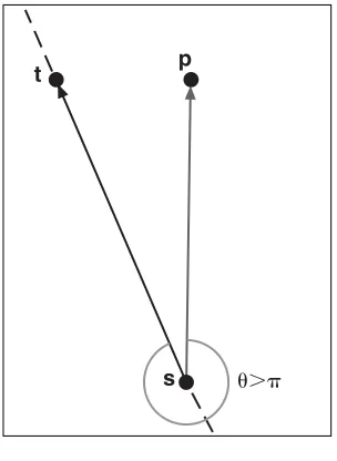
In a 2D world, you can use the cross product to determine the “side” of a vertex given a vector. In other words, if you have a vector, you can determine whether a particular point is to the right or to the left of the vector. To compute this, simply consider the cross prod-uct of the boundary vector (call it st) and consider the vector from point s to your point p sp. You know that the cross product’s direction can tell you whether the vectors are sep-arated by less than . At this point, the deduction should be fairly straightforward; com-pute the cross product ofstwith sp, and if the zcomponent is positive, you know that the counterclockwise angle between the two vectors is less than and hence spis on the left side of the vector st. Conversely, if the sign is negative, it implies an angle greater than
and thus that spis on the right side ofstas shown in Figure 2.8. Figure 2.7
n o t e
The z component of the cross product is also called the determinant, and can be generalized to greater dimensions—a topic you will dive into in the next chapter.
You have studied the cross product’s direction quite a bit, but recall that vectors are ele-ments determined by both direction and magnitude. Not much has been said thus far about the magnitude of the cross product, but there is a reasonably easy formula to deter-mine it (the proof for this one is a rather long and boring algebraic manipulation involv-ing the definition of the norm combined with the definition of the dot product and one trigonometric identity, so I’ll skip that here):
This formula should come as no surprise because it is quite similar to the one for the dot product. You already observed that the direction of the vector generated by the formula Figure 2.8
Using the cross product to determine on which side of a vector a given point exists
was sensitive to angles greater to , and this formula clearly states this fact by inverting the sign for such angles. This also brings up an interesting fact. If you take the cross prod-uct ofsandt, you get a given vector. If you invert the order ofsandt, you are basically changing the angle to (2⫺ ); plugging this value into the equation will make you realize that all this does is invert the sign of the vector. In other words:
There is also a geometrical explanation for the cross product’s length. First, put the two vectors such that their tails match and rotate them equally such that one vector is hori-zontal. Then, add sat the head of t and tat the head of s to generate a parallelogram. Finally, cut off one of the sides’ small triangles and paste it to the other end; you will notice that you have basically built a square. You probably already know how to compute the area of a square (height • width). You already have the width (it is given by the norm oft); you can compute the height because by using the sine identity, you know that it’s sin() times the norm ofs, as illustrated in Figure 2.9. To sum things up, the length of the cross prod-uct is actually the area of the parallelogram generated by the vectors sandt.
t i p
In Maple, the cross product can be computed on two vec-tors by issuing the cross command like so: cross(s+t).
Vector Spaces
The concept of vector spaces is rather interesting because it links vectors with the coordinate sys-tems. A vector space is defined as a set of vectors s,t,u, which have the following properties given any scalar a,b:
Figure 2.9
This set of properties may very well sound quite ridiculous, but believe it or not, there are many other spaces that do not abide by some of these rules. Until now, you have implic-itly used a vector space of {<1, 0, 0>, <0, 1, 0>, <0, 0, 1>}.
Independence Day
If you were expecting to read a few lines about the movie Independence Day, the short answer is that you are not. Rather, this section discusses linear dependency between the vectors.
As you work with vector spaces, it is useless to carry out the same information. Having two equal vectors does not really provide much information to you. As you work with vec-tors, you’ll want to make sure that you do not have the same information twice.
It was previously noted that two vectors are linearly independent if they are not parallel. One way to state the opposite is to say that two vectors are linearly dependent if one vec-tor is a multiple of the other. This stems from the fact that two parallel vecvec-tors must share the same direction, and therefore only the magnitude may change between them. You can also generalize this to say that a set of vectors is linearly dependent if there exists one vec-tor that can be expressed as a linear combination of the others.
The odd term here is “linear combination.” You know that for two vectors to be linearly dependent, one must be a scalar multiple of the other. In the general sense, a linear com-bination is nothing more than the sum of vectors individually multiplied by a scalar. If you think about it for a second, you used linear combinations when you learned about the addition of vectors. An addition is in fact a linear combination. The only trick here is that the vectors were always multiplied by the constant scalar value 1. This definition, howev-er, is not that restrictive. Put in terms of an equation, a linearly dependent set of vectors viadhere to the following condition for one vector vkand with at least one coefficient ai
non-zero:
When you talk about a span, redundancy becomes useless; you can discard any vector that is a linear combination of the others. In other words, the span for the first example of a vector set is no different than if you were to omit the last vector of the set. In fact, you could omit any of the three vectors because any vectors in that set can be expressed as a linear combination of the other two.
Basis
A basis can easily be defined as a minimal set of vectors that can span the entire space. The last example you saw is a basis. A more sophisticated example of a basis would be {<1, 2, 0>, <0, 1, 2>, <1, 0, 2>}. You can verify that this does indeed form a basis by trying to find non-zero scalars a,b, and csuch that the linear combination of these vectors is the vector 0. Finding such a possibility implies that at least one vector can be written as a linear com-bination of the others. Note that this is exactly the same as the linear independence equa-tion stated in the preceding secequa-tion, in which every term was grouped on the same side of the equation. The equation is as follows:
You can juggle the equations as much as you like, but you will never find a non-trivial solution to this problem. Everything comes down to the trivial solution; hence, the set is linearly independent.