Database Management System
by
Vijaykumar Mantri,
Asso. Prof. IT dept,
BVRIT, Narsapur
Index
Unit No
Name
Page No.
Syllabus 1
I Introduction to DBMS 3
II Database Design & ER Diagrams 15
III Relational Model & Relational Algebra 27 IV Structured Query Language (SQL) 66
V Schema Refinement & Normal Forms 85 VI Transactions & Concurrency Control 97
VII Recovery System 115
VIII Overview of Storage and Indexing 127
JAWAHARLAL NEHRU TECHNOLOGICAL UNIVERSITY applications Programs – data base Users and Administrator – Transaction Management – data base System Structure – Storage Manager – the Query Processor
UNIT II : Introduction to Views – Destroying /altering Tables and Views.
Relational Algebra – Selection and projection set operations – renaming – Joins – Division – Examples of Algebra overviews – Relational calculus – Tuple relational Calculus – Domain relational calculus – Expressive Power of Algebra and calculus.
UNIT IV :
Form of Basic SQL Query – Examples of Basic SQL Queries – Introduction to Nested Queries – Correlated Nested Queries Set – Comparison Operators – Aggregative Operators – NULL values – Comparison using Null values – Logical connectivity’s – AND, OR and NOT – Impact on SQL Constructs – Outer Joins – Disallowing NULL values – Complex Integrity Constraints in SQL Triggers and Active Data bases.
UNIT V :
UNIT VI :
Transaction Concept- Transaction State- Implementation of Atomicity and Durability – Concurrent – Executions – Serializability- Recoverability – Implementation of Isolation – Testing for serializability- Lock –Based Protocols – Timestamp Based Protocols- Validation- Based Protocols – Multiple Granularity.
UNIT VII :
Recovery and Atomicity – Log – Based Recovery – Recovery with Concurrent Transactions – Buffer Management – Failure with loss of nonvolatile storage-Advance Recovery systems- Remote Backup systems.
UNIT VIII :
Data on External Storage – File Organization and Indexing – Cluster Indexes, Primary and Secondary Indexes – Index data Structures – Hash Based Indexing – Tree base Indexing – Comparison of File Organizations – Indexes and Performance Tuning- Intuitions for tree Indexes – Indexed Sequential Access Methods (ISAM) – B+ Trees: A Dynamic Index Structure.
TEXT BOOKS :
1. Data base Management Systems, Raghurama Krishnan, Johannes Gehrke, TATA McGrawHill 3rd Edition
2. Data base System Concepts, Silberschatz, Korth, McGraw hill, V edition.
REFERENCES :
1. Data base Systems design, Implementation, and Management, Peter Rob & Carlos Coronel 7th Edition.
2. Fundamentals of Database Systems, Elmasri Navrate Pearson Education 3. Introduction to Database Systems, C.J.Date Pearson Education
4. Oracle for Professionals, The X Team, S Shah and V.Shah,SPD.
Database Management System
Storage Manager – The Query Processor.INTRODUCTION TO DBMS
Introduction :-
Database Management is an important aspect of data processing. It involves, several data models evolving into different DBMS software packages. These packages demand certain knowledge in discipline and procedures to effectively use them in data processing applications. We need to understand the relevance and scope of Database in the Data processing area. This we do by first understanding the properties and characteristics of data and the nature of data organization.A database is a collection of data, typically describing the activities of one or more related organizations. A database is a collection of related information stored in a manner that it is available to many users for different purposes. The content of a database is obtained by combining data from all the different sources in an organization. So that data are available to all users and redundant data can be eliminated or at least minimized.
A database management system, or DBMS, is software designed to assist in maintaining and utilizing large collections of data. The DBMS helps create an environment in which end user have better access to more and better managed data than they did before the DBMS become the data management standard. Most database management systems have the following facilities/capabilities:
Creating of a file, addition to data, deletion of data, modification of data; creation, addition and deletion of entire files.
Retrieving data collectively or selectively.
Database Applications: Banking: all transactions
Airlines: reservations, schedules Universities: registration, grades Sales: customers, products, purchases
Manufacturing: production, inventory, orders, supply chain Human resources: employee records, salaries, tax deductions Databases touch all aspects of our lives.
In the early days, database applications were built on top of file systems
The traditional file-oriented approach to information processing has for each application a separate master file and its own set of personal files. An organization needs flow of information across these applications also and this requires sharing of data, which is significantly lacking in the traditional approach. One major limitations of such a file-based approach is that the programs become dependent on the files and the files become dependent upon the programs.
Disadvantages of File System
Data Redundancy: The same piece of information may be stored in two or more files. For example, the particulars of an individual who may be a customer or client may be stored in two or more files. Some of this information may be changing, such as the address, the payment maid, etc. It is therefore quite possible that while the address in the master file for one application has been updated the address in the master file for another application may have not been. It may be not easy to even find out as to in how many files the repeating items such as the name occur.
Program/Data Dependency: In the traditional approach if a data field is to be added to a master file, all such programs that access the master file would have to be changed to allow for this new field which would have been added to the master record.
Lack of Flexibility: In view of the strong coupling between the program and the data, most information retrieval possibilities would be limited to well-anticipated and pre-determined requests for data, the system would normally be capable of producing scheduled records and queries which it has been programmed to create.
Atomicity of updates : Failures may leave database in an inconsistent state with partial updates carried out. E.g. transfer of funds from one account to another should either complete or not happen at all.
Concurrent access by multiple users Concurrent accessed needed for performance. Uncontrolled concurrent accesses can lead to inconsistencies. E.g. two people reading a balance and updating it at the same time.
Security problems
Database systems offer solutions to all the above problems. The work in the organization may not require significant sharing of data or complex access. In other words the data and the way it is used in the functioning of the organization are not appropriate to database processing. Apart from needing a more powerful hardware platform, the software for database management systems is also quite expensive. This means that a significant extra cost has to be incurred by an organization if it wants to adopt this approach.
Advantages of DBMS
Using a DBMS to manage data has many advantages:
Data Independence: Application programs should not, ideally, be exposed to details of data representation and storage, The DBMS provides an abstract view of the data that hides such details.
Efficient Data Access: A DBMS utilizes a variety of sophisticated techniques to store and retrieve data efficiently. This feature is especially important if the data is stored on external storage devices.
Data Integrity and Security: If data is always accessed through the DBMS, the DBMS can enforce integrity constraints. For example, before inserting salary information for an employee, the DBMS can check that the department budget is not exceeded. Also, it can enforce access controls that govern what data is visible to different classes of users.
Concurrent Access and Crash Recovery: A DBMS schedules concurrent accesses to the data in such a manner that users can think of the data as being accessed by only one user at a time. Further, the DBMS protects users from the effects of system failures.
Reduced Application Development Time: Clearly, the DBMS supports important functions that are common to many applications accessing data in the DBMS. This, in conjunction with the high-level interface to the data, facilitates quick application development. DBMS applications are also likely to be more robust than similar stand-alone applications because many important tasks are handled by the DBMS (and do not have to be debugged and tested in the application).
View of Data : The data in a DBMS is described at three levels of abstraction, as illustrated in
Figure 1.1.
The database description consists of a schema at each of these three levels of abstraction: the Logical (Conceptual), Physical, and View (External).
Physical Level Schema :- The physical schema specifies additional storage details. Essentially, the physical schema summarizes how the relations described in the conceptual schema are actually stored on secondary storage devices such as disks and tapes. It describes how a record (e.g., customer) is stored.
Logical level Schema :- The logical schema (conceptual schema) describes the stored data in terms of the data model of the DBMS. In a relational DBMS, the logical schema describes all relations that are stored in the database. Eg:-
type customer = record name : string; street : string; city : integer; end;
View Level Schema :- View Schemas (External schema), which usually are also in terms of the data model of the DBMS, allow data access to be customized (and authorized) at the level of individual users or groups of users. Any given database has exactly one conceptual schema and one physical schema because it has just one set of stored relations, but it may have several external schemas, each tailored to a particular group of users. Each external schema consists of a collection of one or more views and relations from the conceptual schema.
Instances and Schemas
Schema – The logical structure of the database is called Schema. They are analogous to type information of a variable in a program. e.g., the database consists of information about a set of customers and accounts and the relationship between them.
Physical schema: database design at the physical level Logical schema: database design at the logical level
Instance – The actual content of the database at a particular point in time is called Instance. They are analogous to the value of a variable.
Data Independence
Physical Data Independence– The ability to modify the physical schema without changing the logical schema. Applications depend on the logical schema. In general, the interfaces between the various levels and components should be well defined so that changes in some parts do not seriously influence others.
Data Models
A data model is a collection of high-level data description constructs that hide many low-level storage details. Data models are collection of tools for describing
data
data relationships data semantics data constraints
A DBMS allows a user to define the data to be stored in terms of a data model. Most database management systems today are based on the relational data model. While the data model of the DBMS hides many details, it is nonetheless closer to how the DBMS stores data than to how a user thinks about the underlying enterprise. A semantic data model is a more abstract, high-level data model that makes it easier for a user to come up with a good initial description of the data in an enterprise.
There are several types of data models available.
1. Entity-Relationship Model :- A widely used semantic data model called the entity-relationship (ER) model allows us to pictorially denote entities and the entity-relationships among them. E-R model of real world consists of Entities and Relationships between entities.
Entities (objects) :- E.g. customers, accounts, bank branch
Relationships between entities :- E.g. Account A-101 is held by customer Johnson
E-R Models are widely used for database design. Database design in E-R model usually converted to design in the relational model which is used for storage and processing.
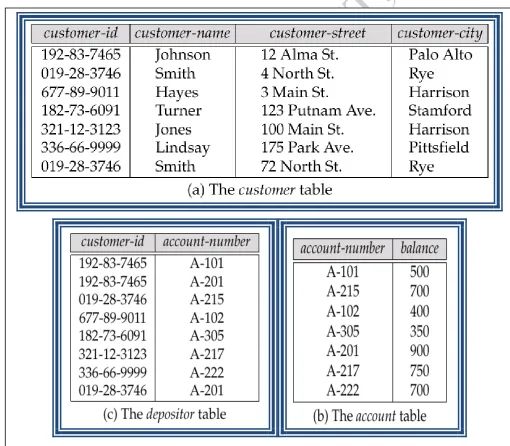
2. Relational model : In this section we provide a brief introduction to the relational model. The central data description construct in this model is a relation, which can be thought of as a set of records. A description of data in terms of a data model is called a schema. In the relational model, the schema for a relation specifies its name, the name of each field (or attribute or column), and the type of each field. The figure 1.3 shows the example of tabular data in the relational model
Other Data Models
In addition to the relational data model (which is used in numerous systems, including IBM's DB2, Informix, Oracle, Sybase, Microsoft's Access, FoxBase, Paradox, Tandem, and Teradata), other important data models include the Hierarchical Model (e.g., used in IBM's IMS DBMS), the network model (e.g., used in IDS and IDMS), the Object-Oriented Model (e.g., used in Objectstore and Versant), and the Object-Relational Model (e.g., used in DBMS products from IBM, Informix, ObjectStore, Oracle, Versant, and others). While many databases use the Hierarchical and Network Models and systems based on the object-oriented and object-relational models are gaining acceptance in the marketplace, the dominant model today is the relational model.
Database Languages :-
Data Definition Language (DDL) :- A data definition language (DDL) is used to define the external and conceptual schemas. It gives specification notation for defining the database schema. This subset of SQL supports the creation, deletion, and modification of definitions for tables and views. Integrity constraints can be defined on tables, either when the table is created or later. E.g. create table account ( account-number char(10), balance integer)
DDL compiler generates a set of tables stored in a data dictionary. Data dictionary contains metadata (i.e., data about data).
There are two classes of languages
Procedural– user specifies what data is required and how to get those data.
Nonprocedural – user specifies what data is required without specifying how to get those data.
SQL :- SQL(Structured Query Language) is the most widely used query language. E.g. find the name of the customer with customer-id 192-83-7465
select customer.customer-name from customer where customer.customer-id = ‗192-83-7465‘ E.g. find the balances of all accounts held by the customer with customer-id 192-83-7465 select account.balance from depositor, account where depositor.customer-id = ‗192
-83-7465‘ and depositor.account-number = account.account-number
Database Access for applications Programs :- Application programs generally access databases through one of
Language extensions to allow embedded SQL
Application program interface (e.g. ODBC/JDBC) which allow SQL queries to be sent to a database
Database Users
Quite a variety of people are associated with the creation and use of databases. Obviously, there are database implementors, who build DBMS software, and end users who wish to store and use data in a DBMS. Users are differentiated by the way they expect to interact with the system.
Application programmers – Application programmers interact with system through DML calls. Database application programmers develop packages that facilitate data access for end users, who are usually not computer professionals, using the host or data languages and software tools that DBMS vendors provide.
Specialized users – Specialized users write specialized database applications that do not fit into the traditional data processing framework.
Naive users– Naive users invoke one of the permanent application programs that have been written previously. E.g. people accessing database over the web, bank tellers, clerical staff, etc.
Database Administrator :Corporate or enterprise-wide databases are typically important
enough and complex enough that the task of designing and maintaining the database is entrusted to a professional, called the database administrator (DBA). DBA coordinates all the activities of
the database system; the database administrator has a good understanding of the enterprise‘s
information resources and needs. The DBA is responsible for many critical tasks:
Design of the Conceptual and Physical Schemas: The DBA is responsible for interacting with the users of the system to understand what data is to be stored in the DBMS and how it is likely to be used. Based on this knowledge, the DBA must design the conceptual schema (decide what relations to store) and the physical schema (decide how to store them).
Security and Authorization: The DBA is responsible for ensuring that unauthorized data access is not permitted. In general, not everyone should be able to access all the data. In a relational DBMS, users can be granted permission to access only certain views and relations.
Data Availability and Recovery from Failures: The DBA must take steps to ensure that if the system fails, users can continue to access as much of the uncorrupted data as possible. The DBA must also work to restore the data to a consistent state.
Database Tuning: Users' needs are likely to evolve with time. The DBA is responsible for modifying the database, in particular the conceptual and physical schemas, to ensure adequate performance as requirements change.
DBA is also responsible for monitoring performance and responding to changes in requirements of the database.
system crashes) and transaction failures. Concurrency-control manager controls the interaction among the concurrent transactions, to ensure the consistency of the database.
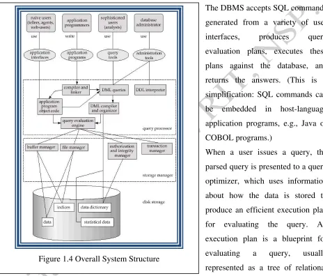
Overall System Structure :-
Figure shows the structure of a typical DBMS based on the relational data model.The DBMS accepts SQL commands generated from a variety of user interfaces, produces query evaluation plans, executes these plans against the database, and returns the answers. (This is a simplification: SQL commands can be embedded in host-language application programs, e.g., Java or COBOL programs.)
When a user issues a query, the parsed query is presented to a query optimizer, which uses information about how the data is stored to produce an efficient execution plan for evaluating the query. An execution plan is a blueprint for evaluating a query, usually represented as a tree of relational operators. Relational operators serve as the building blocks for evaluating queries posed against the data. The code that implements relational operators sits on top of the file and access methods layer. This layer supports the concept of a file, which, in a DBMS, is a collection of pages or a collection of records. Heap files or files of unordered pages, as well as indexes are supported. In addition to keeping track of the pages in a file, this layer organizes the information within a page. The files and access methods layer code sits on top of the buffer manager, which brings pages in from disk to main memory as needed in response to read requests. The lowest layer of the DBMS
software deals with management of space on disk, where the data is stored. Higher layers allocate, deallocate, read, and write pages through (routines provided by) this layer, called the disk space manager. The DBMS supports concurrency and crash recovery by carefully scheduling user requests and maintaining a log of all changes to the database. DBMS components associated with concurrency control and recovery include the transaction manager, which ensures that transactions request and release locks according to a suitable locking protocol and schedules the execution transactions; the lock manager, which keeps track of requests for locks and grants locks on database objects when they become available; and the recovery manager, which is responsible for maintaining a log and restoring the system to a consistent state after a crash. The disk space manager, buffer manager, and file and access method layers must interact with these components.
Storage Management :- Storage manager is a program module that provides the interface
between the low-level data stored in the database and the application programs and queries submitted to the system. The storage manager is responsible to the following tasks:
Interaction with the file manager.
Database Management System
UNIT II
History of Database Systems. Database design and ER diagrams – Beyond ER Design - Entities, Attributes and Entity sets – Relationships and Relationship sets – Additional features of ER Model – Concept Design with the ER Model – Conceptual Design for Large enterprises.
DATABASE DESIGN AND ER DIAGRAMS
Database Design and ER Diagrams
The database design process can be divided into six steps. The ER model is most relevant to the first three steps.
1. Requirements Analysis: The very first step in designing a database application is to understand what data is to be stored in the database, what applications must be built on top of it, and what operations are most frequent and subject to performance requirements. In other words, we must find out what the users want from the database.
2. Conceptual Database Design: The information gathered in the requirements analysis step is used to develop a high-level description of the data to be stored in the database, along with the constraints known to hold over this data. This step is often carried out using the ER model. The ER model is one of several high-level, or semantic, data models used in database design. The goal is to create a simple description of the data that closely matches how users and developers think of the data
3. Logical Database Design: We must choose a DBMS to implement our database design, and convert the conceptual database design into a database schema in the data model of the chosen DBMS. We will consider only relational DBMSs, and therefore, the task in the logical design step is to convert an ER schema into a relational database schema.
Beyond ER Design
we must address security issues and ensure that users are able to access the data they need, but not data that we wish to hide from them.
4. Schema Refinement: The fourth step of database design is to analyze the collection of relations in our relational database schema to identify potential problems, and to refine it. In contrast to the requirements analysis and conceptual design steps, which are essentially subjective, schema refinement can be guided by some elegant and powerful theory.
5. Physical Database Design: In this step, we consider typical expected workloads that our database must support and further refine the database design to ensure that it meets desired performance criteria. This step may simply involve building indexes on some tables and clustering some tables, or it may involve a substantial redesign of parts of the database schema obtained from the earlier design steps.
6. Application and Security Design: Any software project that involves a DBMS must consider aspects of the application that go beyond the database itself. Design methodologies like UML try to address the complete software design and development cycle.
Entities, Attributes and Entity Sets :-
An entity is an object in the real world that is distinguishable from other objects. An entity is described using a set of attributes. An entity set is a collection of similar entities.All entities in a given entity set have the same attributes. For each attribute associated with an entity set, we must identify a domain of possible values. For each entity set, we choose a key. A key is a minimal set of attributes whose values uniquely identify an entity in the set. There could be more than one candidate key; if so, we designate one of them as the primary key. For now we assume that each entity set contains at least one set of attributes that uniquely identifies an entity in the entity set; that is, the set of attributes contains a key.
Relationships and Relationship Sets :-
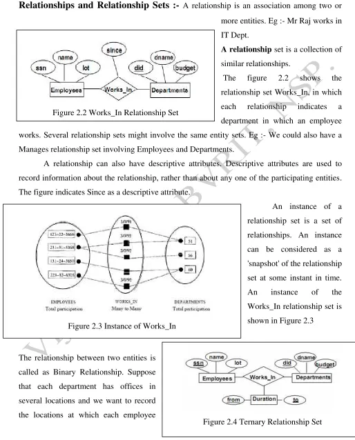
A relationship is an association among two or more entities. Eg :- Mr Raj works in IT Dept.A relationship set is a collection of similar relationships.
The figure 2.2 shows the relationship set Works_In, in which each relationship indicates a department in which an employee works. Several relationship sets might involve the same entity sets. Eg :- We could also have a Manages relationship set involving Employees and Departments.
A relationship can also have descriptive attributes. Descriptive attributes are used to record information about the relationship, rather than about any one of the participating entities. The figure indicates Since as a descriptive attribute.
works. This relationship is Ternary Relationship because we must record an association between an employee, a department, and a location. The ER diagram for this variant of Works_In, which we call Works_In, is shown in Figure.2.4
The entity sets that participate in a relationship set need not be distinct; sometimes a relationship might involve two entities in the same entity set. The example of such entity set is shown in Figure 2.5. If an entity set plays more than one role, the role indicator concatenated with an attribute name from the entity set gives us a unique name for each attribute in the relationship set.
Additional features of ER Model :-
Following are the additional features of ER Model that allow us to describe some subtle properties of the data.
1) Key Constraints :- Consider the Works-.In relationship shown in above figure 2.2. An employee can work in several departments, and a department can have several employees, as illustrated in the Works_In instance shown in above figure 2.3.
single employee is allowed to manage more than one department. The restriction that each department has at most one manager is an example of a key constraint, and it implies that each Departments entity appears in at most one Manages relationship in any allowable instance of Manages. This restriction is indicated in the ER diagram of Figure by using an arrow from Departments to Manages. Intuitively, the arrow states that given a Departments entity, we can uniquely determine the Manages relationship in which it appears.
A relationship set like Manages is sometimes said to be one-to-many, to indicate that one employee can be associated with many departments (in the capacity of a manager), whereas each department can be associated with at most one employee as its manager. In contrast, the Works-In relationship set, in which an employee is allowed to work in several departments and a department is allowed to have several employees, is said to be many-to-many.
The figure 2.7 shows the instance representation of different types of key constraints.
2. Participation Constraints :- The key constraint on Manages tells us that a department has at most one manager. A natural question to ask is whether every department has a manager. Let us say that every department is required to have a manager. This requirement is an example of a participation constraint; the participation of the entity set Departments in the relationship set Manages is said to be total. A participation that is not total is said to be partial. As an example, the participation of the entity set Employees in Manages is partial, since not every employee gets to manage a department. The ER diagram in Figure shows both the Manages and Works_In relationship sets and all the given constraints. If the participation of an entity set in a relationship set is total, the two are connected by a thick line; independently, the presence of an arrow indicates a key constraint.
3. Weak Entities :- Thus far, we have assumed that the attributes associated with an entity set include a key. This assumption does not always hold. For example, suppose that employees can purchase insurance policies to cover their dependents. We wish to record information about policies, including who is covered by each policy, but this information is really our only interest in the dependents of an employee. If an employee quits, any policy owned by the employee is terminated and we want to delete all the relevant policy and dependent information from the database.
Dependents is an example of a weak entity set as shown in figure 2.9. A weak entity can be identified uniquely only by considering some of its attributes in conjunction with the primary key of another entity, which is called the identifying owner.
The following restrictions must hold:
1) The owner entity set and the weak entity set must participate in a one-to-many relationship set (one owner entity is associated with one or more weak entities, but each weak entity has a single owner). This relationship set is called the identifying relationship set of the weak entity set.
Figure 2.8 Manages & Works_In
2) The weak entity set must have total participation in the identifying relationship set. For example, a Dependents entity can be identified uniquely only if we take the key of the owning Employees entity and the pname of the Dependents entity.
The set of attributes of a weak entity set that uniquely identify a weak entity for a given owner entity is called a partial key of the weak entity set. In our example, pname is a partial key for Dependents.
4. Class Hierarchies :- Sometimes it is natural to classify the entities in an entity set into subclasses.
For example, we might want to talk about an Hourly_Emps entity set and a Contract_Emps entity set to distinguish the basis on which they are paid. We might have attributes hours_worked and hourly_wage defined for Hourly_Emps and an attribute contractid defined for Contract_Emps. This gives us a scenario that the attributes for the entity set Employees are inherited by the
entity set
Solution to selected exercises
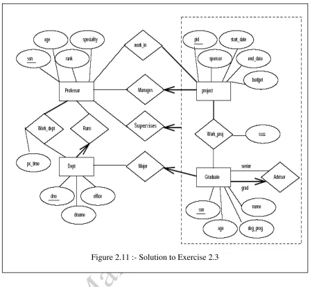
Exercise 2.3 Consider the following information about a university database: Professors have an SSN, a name, an age, a rank, and a research specialty.
Projects have a project number, a sponsor name (e.g., NSF), a starting date, an ending date, and a budget.
Graduate students have an SSN, a name, an age, and a degree program (e.g., M.S. or Ph.D.).
Each project is managed by one professor (known as the project's principal investigator). Each project is worked on by one or more professors (known as the project's
co-investigators).
Professors can manage and/or work on multiple projects.
Each project is worked on by one or more graduate students (known as the project's research assistants).
When graduate students work on a project, a professor must supervise their work on the project. Graduate students can work on multiple projects, in which case they will have a (potentially different) supervisor for each one.
Departments have a department number, a department name, and a main office. Departments have a professor (known as the chairman) who runs the department.
Professors work in one or more departments and for each department that they work in, a time percentage is associated with their job.
Graduate students have one major department in which they are working on their degree. Each graduate student has another, more senior graduate student (known as a student
advisor) who advises him or her on what courses to take.
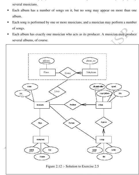
Exercise 2.5 Notown Records has decided to store information about musicians who perform on its albums (as well as other company data) in a database. The company has wisely chosen to hire you as a database designer (at your usual consulting fee of $2500/day).
Each musician that records at Notown has an SSN, a name, an address, and a phone number. Poorly paid musicians often share the same address, and no address has more than one phone.
Each instrument used in songs recorded at Notown has a unique identification number, a name (e.g., guitar, synthesizer, flute) and a musical key (e.g., C, B-flat, E-flat).
Each album recorded on the Notown label has a unique identification number, a title, a copyright date, a format (e.g., CD or MC), and an album identifier.
Each musician may play several instruments, and a given instrument may be played by several musicians.
Each album has a number of songs on it, but no song may appear on more than one album.
Each song is performed by one or more musicians, and a musician may perform a number of songs.
Each album has exactly one musician who acts as its producer. A musician may produce several albums, of course.
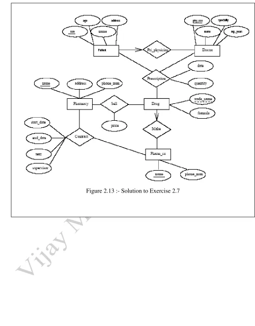
Exercise 2.7 The Prescriptions-R-X chain of pharmacies has offered to give you a free lifetime supply of medicine if you design its database. Given the rising cost of health care, you agree.
Here‘s the information that you gather:
Patients are identified by an SSN, and their names, addresses, and ages must be recorded. Doctors are identified by an SSN. For each doctor, the name, specialty, and years of
experience must be recorded.
Each pharmaceutical company is identified by name and has a phone number.
For each drug, the trade name and formula must be recorded. Each drug is sold by a given pharmaceutical company, and the trade name identifies a drug uniquely from among the products of that company. If a pharmaceutical company is deleted, you need not keep track of its products any longer.
Each pharmacy has a name, address, and phone number.
Every patient has a primary physician. Every doctor has at least one patient.
Each pharmacy sells several drugs and has a price for each. A drug could be sold at several pharmacies, and the price could vary from one pharmacy to another.
Doctors prescribe drugs for patients. A doctor could prescribe one or more drugs for several patients, and a patient could obtain prescriptions from several doctors. Each prescription has a date and a quantity associated with it. You can assume that, if a doctor prescribes the same drug for the same patient more than once, only the last such prescription needs to be stored. Pharmaceutical companies have long-term contracts with pharmacies. A pharmaceutical
company can contract with several pharmacies, and a pharmacy can contract with several pharmaceutical companies. For each contract, you have to store a start date, an end date, and the text of the contract.
Pharmacies appoint a supervisor for each contract. There must always be a supervisor for each contract, but the contract supervisor can change over the lifetime of the contract.
1. Draw an ER diagram that captures the preceding information. Identify any constraints not captured by the ER diagram.
Database Management System
UNIT III
Introduction to the Relational Model – Integrity Constraint over relations – Enforcing Integrity constraints – Querying relational data – Logical data base Design – Introduction to Views – Destroying /altering Tables and Views.
Relational Algebra – Selection and Projection Set operations – Renaming – Joins – Division – Examples of Algebra overviews – Relational calculus – Tuple Relational Calculus – Domain Relational Calculus – Expressive Power of Algebra and calculus.
RELATIONAL MODEL & RELATIONAL ALGEBRA
Introduction to the Relational Model :-
Codd proposed the relational data model in 1970. The relational model is by far the dominant data model and the foundation for the leading DBMS products, including IBM's DB2 family, Informix, Oracle, Sybase, Microsoft's Access and SQLServer, FoxBase, and Paradox.
The relational model is very simple and elegant: a database is a collection of one or more relations, where each relation is a table with rows and columns. The main construct for representing data in the relational model is a relation.
A relation consists of a relation schema and a relation instance. The relation instance is a table, and the relation schema describes the column heads for the table. We first describe the relation schema and then the relation instance. The schema specifies the relation's name, the name of each field (or column, or attribute), and the domain of each field. A domain is referred to in a relation schema by the domain name and has a set of associated values.
We use the example of student information in a university database to illustrate the parts of a relation schema:
Students(sid: string, name: string, login: string, age: integer, gpa: real)
There is a requirement of the relational model-each relation is defined to be a set of unique tuples or rows as well as the order in which the rows are listed is not important.
A relation schema specifies the domain of each field or column in the relation instance. These domain constraints in the schema specify an important condition that we want each instance of the relation to satisfy: The values that appear in a column must be drawn from the domain associated with that column. Thus, the domain of a field is essentially the type of that field, in programming language terms, and restricts the values that can appear in the field.
Domain constraints are so fundamental in the relational model that we henceforth consider only relation instances that satisfy them; therefore, relation instance means relation instance that satisfies the domain constraints in the relation schema.
The degree, also called arity, of a relation is the number of fields. The cardinality of a relation instance is the number of tuples in it.
In Figure 3.1, the degree of the relation (the number of columns) is five, and the cardinality of this instance is three.
A relational database is a collection of relations with distinct relation names. The relational database schema is the collection of schemas for the relations in the database.
Relational Query Language
Creating and Modifying Relations Using SQL
The SQL language standard uses the word table to denote relation, and we often follow this convention when discussing SQL. The subset of SQL that supports the creation, deletion, and modification of tables is called the Data Definition Language (DDL). Further, while there is a
command that lets users define new domains, analogous to type definition commands in a programming language. We only consider domains that are built-in types, such as integer. The CREATE TABLE statement is used to define a new table. To create the Students relation, we can use the following statement:
CREATE TABLE Students ( sid CHAR(20), name CHAR(30), login CHAR(20), age INTEGER, gpa REAL)
Tuples are inserted, using the INSERT command. We can insert a single tuple into the Students table as follows:
INSERT INTO Students (sid, name, login, age, gpa) VALUES (536, 'Smith', 'smith@ee', 18, 3.2) We can optionally omit the list of column names in the INTO clause and list the values in the appropriate order, but it is good style to be explicit about column names.
We can delete tuples using the DELETE command. We can delete all Students tuples with name equal to Smith using the command:
DELETE FROM WHERE Students S S.name = 'Smith'
We can modify the column values in an existing row using the UPDATE command. For example, we can increment the age and decrement the gpa of the student with sid 536: UPDATE Students S SET S.age = S.age + 1, S.gpa = S.gpa – 1 WHERE S.sid = 536
These examples illustrate some important points. The WHERE clause is applied first and determines which rows are to be modified. The SET clause then determines how these rows are to be modified. If the column being modified is also used to determine the new value, the value used in the expression on the right side of equals (=) is the old value, that is, before the modification.
Integrity Constraint over Relations :-
Many kinds of integrity constraints can be specified in the relational model.
Key Constraints :- Consider the Students relation and the constraint that no two students have the same student id. This IC is an example of a key constraint. A key constraint is a statement that a certain minimal subset of the fields of a relation is a unique identifier for a tuple. A set of fields that uniquely identifies a tuple according to a key constraint is called a candidate key for the relation; we often abbreviate this to just key. In the case of the Students relation, the (set of fields containing just the) sid field is a candidate key.
Every relation is guaranteed to have a key. Since a relation is a set of tuples, the set of all fields is always a superkey. If other constraints hold, some subset of the fields may form a key, but if not, the set of all fields is a key. A relation may have several candidate keys. Out of all the available candidate keys, a database designer can identify a primary key. Intuitively, a tuple can be referred to from elsewhere in the database by storing the values of its primary key fields. For example, we can refer to a Students tuple by storing its sid value.
Specifying Key Constraints in SQL
In SQL, we can declare that a subset of the columns of a table constitute a key by using the UNIQUE constraint. At most one of these candidate keys can be declared to be a primary key, using the PRIMARY KEY constraint. (SQL does not require that such constraints be declared for a table.)
We will rewrite Students table definition and specify key information:
CREATE TABLE Students ( sid CHAR(20), name CHAR (30), login CHAR(20), age
INTEGER, gpa REAL, UNIQUE (name, age), CONSTRAINT StudentsKey PRIMARY KEY (sid) )
This definition says that sid is the primary key and the combination of name and age is also a key. The definition of the primary key also illustrates how we can name a constraint by preceding it with CONSTRAINT constraint-name. If the constraint is violated, the constraint name is returned and can be used to identify the error.
Foreign Key Constraints
modified, to keep the data consistent. An IC involving both relations must be specified if a DBMS is to make such checks. The most common IC involving two relations is a foreign key constraint. Suppose that, in addition to Students, we have a second relation:
Enrolled(studid: string, cid: string, grade: string)
To ensure that only bonafide students can enroll in courses, any value that appears in the studid field of an instance of the Enrolled relation should also appear in the sid field of some tuple in the Students relation. The studid field of Enrolled is called a foreign key and refers to Students.
Specifying Foreign Key Constraints in SQL
Let us define Enrolled(studid: string, cid: string, grade: string):
CREATE TABLE Enrolled ( studid CHAR(20), cid CHAR(20), grade CHAR(10), PRIMARY KEY (studid, cid), FOREIGN KEY (studid) REFERENCES Students)
The foreign key constraint states that every studid value in Enrolled must also appear in Students, that is, studid in Enrolled is a foreign key referencing Students.
Enforcing Integrity constraints :-
ICs are specified when a relation is created and enforced when a relation is modified. The impact of domain, PRIMARY KEY, and UNIQUE constraints is straightforward: If an insert, delete, or update command causes a violation, it is rejected. Every potential IC violation is generally checked at the end of each SQL statement execution, although it can be deferred until the end of the transaction executing the statement.
If insertion violates the primary key constraint it will be rejected by the DBMS. Deletion does not cause a violation of constraint, primary key or unique constraints. However, an update can cause violations, similar to an insertion. The impact of foreign key constraints is more complex because SQL sometimes tries to rectify a foreign key constraint violation instead of simply rejecting the change.
CREATE TABLE Enrolled ( studid CHAR(20), cid CHAR(20), grade CHAR(10), PRIMARY KEY (studid, cid), FOREIGN KEY (studid) REFERENCES Students ON DELETE CASCADE ON UPDATE NO ACTION)
The options are specified as part of the foreign key declaration. The default option is NO ACTION, which means that the action (DELETE or UPDATE) is to be rejected, Thus, the ON UPDATE clause in our example could be omitted, with the same effect. The CASCADE keyword says that, if a Students row is deleted, all Enrolled rows that refer to it are to be deleted as well. If the UPDATE clause specified CASCADE, and the sid column of a Students row is updated, this update is also carried out in each Enrolled row that refers to the updated Students row. If a Students row is deleted, we can switch the enrollment to a 'default' student by using ON DELETE SET DEFAULT. SQL also allows the use of null as the default value by specifying ON DELETE SET NULL.
Querying Relational Data
A relational database query (query, for short) is a question about the data, and the answer consists of a new relation containing the result. For example, we might want to find all students younger than 18 or all students enrolled in Reggae203. A query language is a specialized language for writing queries. SQL is the most
popular commercial query language for a
SELECT * FROM Students S WHERE S.age < 18 The result of query is shown in figure 3.2
Logical Database Design :-
Following are the ways to translate an ER diagram into a collection of tables with associated constraints, that is, a relational database schema.
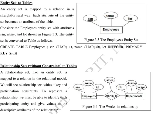
Entity Sets to Tables
An entity set is mapped to a relation in a straightforward way: Each attribute of the entity set becomes an attribute of the table.
Consider the Employees entity set with attributes ssn, name, and lot shown in Figure 3.3. The entity set is converted to Table as follows.
CREATE TABLE Employees ( ssn CHAR(11), name CHAR(30), lot INTEGER, PRIMARY KEY (ssn))
Relationship Sets (without Constraints) to Tables A relationship set, like an entity set, is mapped to a relation in the relational model. We will see relationship sets without key and participation constraints. To represent a relationship, we must be able to identify each participating entity and give values to the descriptive attributes of the relationship. Thus, the attributes of the relation include:
• The primary key attributes of each participating entity set, as foreign key fields. • The descriptive attributes of the relationship set.
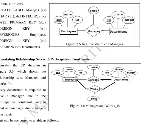
Consider the Works_in relationship as shown in figure 3.4. This relationship set is converted to table as follows.
CREATE TABLE Works_In ( ssn CHAR(11), did INTEGER, since DATE, PRIMARY KEY (ssn, did), FOREIGN KEY (ssn) REFERENCES Employees, FOREIGN KEY (did) REFERENCES Departments)
Translating Relationship Sets with Key Constraints
If a relationship set involves n entity sets and some of them are linked via arrows in the ER diagram, the key for anyone of these m entity sets constitutes a key for the relation to which the
Figure 3.3 The Employees Entity Set
relationship set is mapped. Hence we have m candidate keys, and one of these should be designated as the primary key. Consider the Manages relationship set with key constraint (Each department has at most One Manager)as shown in figure 3.5. This relationship set is converted to table as follows. relationship sets, Manages and Works_In.
Every department is required to have a manager, due to the participation constraint, and at most one manager, due to the key constraint.
This can be converted to a table as follows.
CREATE TABLE DeptMgr ( did INTEGER, dname CHAR(20), budget REAL, ssn CHAR(11) NOT NULL, since DATE, PRIMARY KEY (did), FOREIGN KEY (ssn) REFERENCES Employees ON DELETE NO ACTION)
Unfortunately, there are many participation constraints that we cannot capture using SQL.
Translating Weak Entity Sets A weak entity set always participates in a one-to-many
Figure 3.5 Key Constraints on Manages
Figure 3.6 Manages and Works_In
binary relationship and has a key constraint and total participation. We must take into account that the weak entity has only a partial key. Also, when an owner entity is deleted, we want all owned weak entities to be deleted. Consider the Dependents weak entity set shown in Figure 3.7, with partial key pname. A Dependents entity can be identified uniquely only if we take the key of the owning Employees entity and the pname of the Dependents entity and the Dependents entity must be deleted if the owning Employees entity is deleted. Following is the conversion of Dependents Weak entity into a table
CREATE TABLE Dep_Policy (pname CHAR(20), age INTEGER, cost REAL, ssn CHAR (11), PRIMARY KEY (pname, ssn), FOREIGN KEY (ssn) REFERENCES Employees ON DELETE CASCADE) Hourly_Emps here; ContracLEmps is handled similarly. The relation for Hourly_Emps includes the hourly_wages and hours_worked attributes of
Hourly_Emps. It also contains the key attributes of the superclass (ssn, in this example), which serve as the primary key for Hourly_Emps, as well as a foreign key referencing the superclass (Employees). For each Hourly_Emps entity, the value of the name and lot attributes is stored in the corresponding row of the superclass (Employees). Note that if the superclass tuple is deleted, the delete must be cascaded to Hourly_Emps.
2. Alternatively, we can create just two relations, corresponding to Hourly_Emps and Contracrt_Emps. The relation for Hourly_Emps includes all the attributes of Hourly_Emps as well as all the attributes of Employees (i.e., ssn, name, lot, hourly_wages, hours_worked).
Introduction to Views :-
A view is a table whose rows are not explicitly stored in the database but are computed as needed from a view definition. Consider the Students and Enrolled relations. Suppose we are often interested in finding the names and student identifiers of students who got a grade of B in some course, together with the course identifier. We can define a view for this purpose. Using SQL notation:
CREATE VIEW B_Students (name, sid, course) AS SELECT S.sname, S.sid, E.cid FROM Students S, Enrolled E WHERE S.sid = E.studid AND E.grade = 'B'
This view can be used just like a base table, or explicitly stored table, in defining new queries or views.
Destroying/Altering Tables and Views
If we decide that we no longer need a base table and want to destroy it (i.e. delete all the rows and remove the table definition information), we can use the DROP TABLE command. For example, DROP TABLE Students RESTRICT destroys the Students table unless some view or integrity constraint refers to Students; if so, the command fails. If the keyword RESTRICT is replaced by CASCADE, Students is dropped and any referencing views or integrity constraints are (recursively) dropped as well; one of these keywords must always be specified. A view can be dropped using the DROP VIEW command, which is just like DROP TABLE. ALTER TABLE modifies the structure of an existing table. To add a column called maiden-name to Students, for example, we would use the following command:
ALTER TABLE Students ADD COLUMN maiden-name CHAR(10)
Relational Algebra :-
We have two formal query languages associated with the relational model. Query languages are specialized languages for asking questions, or queries that involve the data in a database. Queries in relational algebra are composed using a collection of operators, and each query describes a step-by-step procedure for computing the desired answer; that is, queries are specified in an operational manner.
The inputs and outputs of a query are relations. A query is evaluated using instances of each input relation and it produces an instance of the output relation. We will use field names to refer to fields because this notation makes queries more readable. An alternative is to always list the fields of a given relation in the same order and refer to fields by position rather than by field name. In defining relational algebra and calculus, the alternative of referring to fields by position is more convenient than referring to fields by name: Queries often involve the computation of intermediate results, which are themselves relation instances; and if we use field names to refer to fields, the definition of query language constructs must specify the names of fields for all intermediate relation instances. This can be tedious and is really a secondary issue, because we can refer to fields by position anyway. On the other hand, field names make queries more readable.
We use following Schemas for sample queries
1. Sailors(sid:integer, sname:string, rating:integer, age:real) 2. Boats(bid:integer, bname:string, color:string)
3. Reserves(sid:integer, bid:integer, day:date)
Sid Sname Rating Age
Figure 3.9 Instances of Sailors, Boats & Reserve Selection and Projection
Relational algebra includes operators to select rows from a relation (σ) and to project columns
(π). These operations allow us to manipulate data in a single relation. Consider the instance of the Sailors relation shown in Figure 3.9, denoted as S2. We can retrieve rows corresponding to expert sailors by using the σ operator.
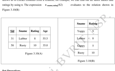
The expression σ rating>8(S2) evaluates to the relation shown in Figure 3.10(A). The
subscript rating> 8 specifies the selection criterion to be applied while retrieving tuples.
can be by position (of the form .i or i) or by name (of the form .name or name). The schema of
the result of a selection is the schema of the input relation instance. The projection operator π
allows us to extract columns from a relation; for example, we can find out all sailor names and
ratings by using π. The expression πsname,rating(S2) evaluates to the relation shown in
Figure 3.10(B)
The following standard operations on sets are also available in relational algebra: union (U), intersection (∩), set-difference (-), and cross-product (X).
1) Union: R U S returns a relation instance containing all tuples that occur in either relation instance R or relation instance S (or both). R and S must be union-compatible, and the schema of the result is defined to be identical to the schema of R.
Two relation instances are said to be union-compatible if the following conditions hold: - They have the same number of the fields, and
- Corresponding fields, taken in order from left to right, have the same domains.
Note that field names are not used in defining union-compatibility. For convenience, we will assume that the fields of R U S' inherit names from R, if the fields of R have names.
3) Set-difference: R - S returns a relation instance containing all tuples that occur in R but not in S. The relations R and S must be union-compatible, and the schema of the result is defined to be identical to the schema of R.
4) Cross-product: R X S returns a relation instance whose schema contains all the fields of R (in the same order as they appear in R) followed by all the fields of S (in the same order as they appear in S). The result of R X S contains one tuple (r, s) (the concatenation of tuples r and s) for each pair of tuples r R, s S. The cross-product operation is sometimes called Cartesian product.
Figure 3.11 illustrate output of these definitions through examples.
Renaming :- We have been careful to adopt field name conventions that ensure that the result of a relational algebra expression inherits field names from its argument (input) relation instances in a natural way whenever possible. However, name conflicts can arise in some cases; for example, in S1 X R1. It is therefore convenient to be able to give names explicitly to the fields of a relation instance that is defined by a relational algebra expression. In fact, it is often convenient to give the instance itself a name so that we can break a large algebra expression into smaller pieces by giving names to the results of subexpressions.
We can use renaming operator ρ for this purpose. The expression ρ (R(F), E) takes an arbitrary relational algebra expression E and returns an instance of a (new) relation called R. R contains the same tuples as the result of E and has the same schema as E, but some fields are renamed. The field names in relation R are the same as in E, except for fields renamed in the Renaming list F, which is a list of terms having the form oldname newname or position newname. For ρ
to be well-defined references to fields (in the form of oldnames or positions in the renaming list) may be unambiguous and no two fields in the result may have the same name.
For example, the expression ρ (C(1sid1, 5sid2),S1 X R1) returns a relation that has the following schema:
C(sid1: integer, sname: string, rating: integer, age: real, sid2:integer, bid: integer, day: date).
Joins
The join operation is one of the most useful operations in relational algebra and the most commonly used way to combine information from two or more relations. Although a join can be defined as a product followed by selections and projections. Further, the result of a cross-product is typically much larger than the result of a join. There are several variants of the join operation.
Condition Joins
The most general version of the join operation accepts a join condition c and a pair of relation instances as arguments and returns a relation instance. The join condition is identical to a selection condition in form. The operation is defined as follows:
Sid Sname Rating Age Bid Day
22 Dustin 7 45.0 103 11/12/96
31 Lubber 8 55.5 103 11/12/96
Figure 3.13 S1
⋈
R.Sid=S.Sid R1Thus join is defined to be a cross-product followed by a selection. Note that the condition c can refer to attributes of both Rand S..
As an example, the result of Sl S1.Sid<R1.Sid R1 is shown in Figure 3.12.
Equijoin
A common special case of the join operation R
⋈
S is when the join condition consists solely of equalities of the form R.name1 = S.name2, that is, equalities between two fields in R and S. In this case, obviously, there is some redundancy in retaining both attributes in the result. For join conditions that contain only such equalities, the join operation is refined by doing an additional projection in which S.name2 is dropped. The join operation with this refinement is called equijoin.We illustrate S1
⋈
R.Sid=S.Sid R1 in Figure 3.13. Note that only one field called sid appears in theresult.
Natural Join
A further special case of the join operation R
⋈
S is an equijoin in which equalities are specified on all fields having the same name in R and S. In this case, we can simply omit the join condition; the default is that the join condition is a collection of equalities on all common fields. We call this special case a natural join, and it has the nice property that the result is guaranteed not to have two fields with the same name.Sid Sname Rating Age (Sid) Bid Day
22 Dustin 7 45.0 58 103 11/12/96
31 Lubber 8 55.5 58 103 11/12/96
Division
The division operator is useful for expressing certain kinds of queries for example, "Find the names of sailors who have reserved all boats." Understanding how to use the basic operators of the algebra to define division is a useful exercise. However, the division operator does not have the same importance as the other operators-it is not needed as often, and database systems do not try to exploit the semantics of division by implementing it as a distinct operator.
Consider two relation instances A and B in which A has (exactly) two fields X and Y and B has just one field Y, with the same domain as in A. We define the division operation A/B as the set of all X values (in the form of unary tuples) such that for every Y value in (a tuple of) B, there is a tuple (X,Y) in A.
Division is illustrated in Figure 3.14.
Relational Calculus
Relational calculus is an alternative to relational algebra. In contrast to the algebra, which is procedural, the calculus is nonprocedural, or declarative, in that it allows us to describe the set of answers without being explicit about how they should be computed. Relational calculus has had a big influence on the design of commercial query languages such as SQL and, especially, Query-By-Example (QBE).
The first variant is called the tuple relational calculus (TRC). Variables in TRC take on tuples as values. In another variant, called the domain relational calculus (DRC), the variables range over field values.
Tuple Relational Calculus
A tuple variable is a variable that takes on tuples of a particular relation schema as values. That is, every value assigned to a given tuple variable has the same number and type of fields. A tuple relational calculus query has the form { T I p(T) }, where T is a tuple variable and p(T) denotes a formula that describes T.
• Let Rel be a relation name, R and S be tuple variables, a be an attribute of R, and b be an attribute of S.
• Let op denote an operator in the set {<, >, =, >=, <=, <>}.
• An atomic formula in TRC is one of the following:
– R ∈Rel
– R.a op S.b
– R.a op constant, or constant op R.a
A formula is recursively defined to be one of the following, where p and q are themselves formulas and p(R) denotes a formula in which the variable R appears:
• any atomic formula
• ¬p, p q, p vq, or p ⇒q
• ∃R(p(R)), where Ris a tuple variable.
Examples
• Find the names and ages of sailors with a rating above 7.
{P I S Sailors(S.rating > 7 P.name = S.sname P.age = S.age)}
• Find the sailor name, boatid, and reservation date for each reservation. {P I R Reservation S Sailors
(R.sid = S.sid P.bid = R.bid P.day = R.day P.sname = S.sname)}
• Find the names of sailors who have reserved all boats. {P I S Sailors B Boats
( R Reserves(S.sid = R.sid R.bid = B.bid Psname = S.sname))}
• Find sailors who have reserved all red boats. {S I S Sailors B Boats (B.color ='red' ( R Reserves( S.sid = R.sid R.bid = B.bid)))}
Domain Relational Calculus
A domain variable is a variable that ranges over the values in the domain of some attribute (e.g., the variable can be assigned an integer if it appears in an attribute whose domain is the set of integers).
A DRC query has the form
{ <XI,X2, ... ,Xn > | p(<XI,X2, ... ,Xn >)}
where each Xi is either a domain variable or a constant and p( <Xl, X2, ... ,Xn >) denotes a DRC formula whose only free variables are the variables among the Xi, 1 <= i <=n . The result of this query is the set of all tuples <Xl, X2, ., X n> for which the formula evaluates to true.
• A DRC formula is defined in a manner very similar to the definition of a TRC formula.
• The main difference is that the variables are now domain variables.
A formula is recursively defined to be one of the following, where p and q are themselves formulas and p(X) denotes a formula in which the variable X appears:
• any atomic formula
• ¬p, p ^ q, p V q, or p ⇒q
• ∃X(p(X)), where X is a domain variable
• ∀X(p(X)), where X is a domain variable
Examples
• Find all sailors with a rating above 7.
{<I, N, T, A> | <I, N, T, A> Sailors T > 7}
• Find the names of sailors who have reserved boat 103.
Solution to selected exercises
Exercise 3.11 Suppose that we have a ternary relationship R between entity sets A, B, and C such that A has a key constraint and total participation and B has a key constraint; these are the only constraints. A has attributes a1 and a2, with a1 being the key; B and C are similar. R has no descriptive attributes. Write SQL statements that create tables corresponding to this information so as to capture as many of the constraints as possible. If you cannot capture some constraint, explain why.
Answer 3.11 The following SQL statements create the corresponding relations.
CREATE TABLE A ( a1 CHAR(10), a2 CHAR(10), b1 CHAR(10), c1 CHAR(10), PRIMARY KEY (a1), UNIQUE (b1), FOREIGN KEY (b1) REFERENCES B, FOREIGN KEY (c1) REFERENCES C )
CREATE TABLE B ( b1 CHAR(10), b2 CHAR(10), PRIMARY KEY (b1) ) CREATE TABLE C ( b1 CHAR(10), c2 CHAR(10), PRIMARY KEY (c1) )
The first SQL statement folds the relationship R into table A and thereby guarantees the participation constraint.
Exercise 3.13 Consider the university database from Exercise 2.3 and the ER diagram you designed. Write SQL statements to create the corresponding relations and capture as many of the constraints as possible. If you cannot capture some constraints, explain why.
Answer 3.13 The following SQL statements create the corresponding relations.
1. CREATE TABLE Professors ( prof ssn CHAR(10), name CHAR(64), age INTEGER, rank INTEGER, speciality CHAR(64), PRIMARY KEY (prof ssn) )
2. CREATE TABLE Depts ( dno INTEGER, dname CHAR(64), office CHAR(10), PRIMARY KEY (dno) )
3. CREATE TABLE Runs ( dno INTEGER, prof ssn CHAR(10), PRIMARY KEY ( dno, prof ssn), FOREIGN KEY (prof ssn) REFERENCES Professors, FOREIGN KEY (dno)
REFERENCES Depts )