Know It All
AMSTERDAM • BOSTON • HEIDELBERG • LONDON NEW YORK • OXFORD • PARIS • SAN DIEGO SAN FRANCISCO • SINGAPORE • SYDNEY • TOKYO
Morgan Kaufmann is an imprint of Elsevier
Stephen Buxton
Lowell Fryman
Ralf Hartmut Güting
Terry Halpin
Jan L. Harrington
William H. Inmon
Sam S. Lightstone
Jim Melton
Tony Morgan
Thomas P. Nadeau
Bonnie O’Neil
Elizabeth O’Neil
Patrick O’Neil
Markus Schneider
Graeme Simsion
Toby J. Teorey
This book is printed on acid-free paper.
Copyright © 2009 by Elsevier Inc. All rights reserved.
Designations used by companies to distinguish their products are often claimed as trademarks or registered trademarks. In all instances in which Morgan Kaufmann Publishers is aware of a claim, the product names appear in initial capital or all capital letters. Readers, however, should contact the appropriate companies for more complete information regarding trademarks and registration.
No part of this publication may be reproduced, stored in a retrieval system, or transmitted in any form or by any means, electronic, mechanical, photocopying, scanning, or otherwise, without prior written permission of the publisher.
Permissions may be sought directly from Elsevier’s Science & Technology Rights Department in Oxford, UK: phone: (+44) 1865 843830, fax: (+44) 1865 853333, e-mail: permissions@elsevier.com. You may also complete your request on-line via the Elsevier homepage (http://elsevier.com), by selecting “Support & Contact” then “Copyright and Permission” and then “Obtaining Permissions.”
Library of Congress Cataloging-in-Publication Data Teorey, Toby J.
Database design : know it all / Toby Teorey et al. p. cm. — (Morgan Kaufmann know it all series) Includes index.
ISBN 978-0-12-374630-6 (alk. paper) 1. Database design. I. Title. QA76.9.D26T42 2008
005.74—dc22 2008040366
For information on all Morgan Kaufmann publications,
visit our Website at www.mkp.com or www.books.elsevier.com Printed in the United States
08 09 10 11 12 10 9 8 7 6 5 4 3 2 1
Working together to grow
libraries in developing countries
About This Book ... ix
Contributing Authors ... xi
CHAPTER 1
Introduction
... 11.1 Data and Database Management ... 1
1.2 The Database Life Cycle ... 2
1.3 Conceptual Data Modeling ... 7
1.4 Summary ... 9
1.5 Literature Summary ... 9
CHAPTER 2
Entity–Relationship Concepts
... 112.1 Introduction to ER Concepts ... 13
2.2 Further Details of ER Modeling ... 20
2.3 Additional ER Concepts ... 29
2.4 Case Study ... 32
2.5 Normalization: Preliminaries ... 36
2.6 Functional Dependencies ... 41
2.7 Lossless Decompositions ... 57
2.8 Normal Forms ... 65
2.9 Additional Design Considerations... 80
2.10 Suggestions for Further Reading... 83
CHAPTER 3
Data Modeling in UML
... 853.1 Introduction ... 85
3.2 Object Orientation ... 88
3.3 Attributes... 91
3.4 Associations ... 97
3.5 Set-Comparison Constraints ... 105
3.6 Subtyping ... 113
3.7 Other Constraints and Derivation Rules ... 118
3.8 Mapping from ORM to UML ... 132
3.9 Summary ... 136
CHAPTER 4
Requirements Analysis and Conceptual
Data Modeling
... 1414.1 Introduction ... 141
4.2 Requirements Analysis ... 142
4.3 Conceptual Data Modeling ... 143
4.4 View Integration ... 152
4.5 Entity Clustering for ER Models ... 160
4.6 Summary ... 165
4.7 Literature Summary ... 167
CHAPTER 5
Logical Database Design
... 1695.1 Introduction ... 169
5.2 Overview of the Transformations Required ... 170
5.3 Table Specifi cation ... 172
5.4 Basic Column Defi nition ... 181
5.5 Primary Key Specifi cation ... 187
5.6 Foreign Key Specifi cation ... 189
5.7 Table and Column Names ... 200
5.8 Logical Data Model Notations ... 201
5.9 Summary ... 203
CHAPTER 6
Normalization
... 2056.1 Translating an ER Diagram into Relations ... 205
6.2 Normal Forms ... 206
6.3 First Normal Form ... 207
6.4 Second Normal Form ... 212
6.5 Third Normal Form ... 214
6.6 Boyce-Codd Normal Form ... 216
6.7 Fourth Normal Form ... 217
6.8 Normalized Relations and Database Performance ... 219
6.9 Further Reading ... 224
CHAPTER 7
Physical Database Design
... 2257.1 Introduction ... 225
7.2 Inputs to Database Design ... 226
7.3 Options Available to the Database Designer ... 228
7.4 Design Decisions that Do Not Affect Program Logic ... 229
7.5 Crafting Queries to Run Faster ... 237
7.6 Logical Schema Decisions ... 238
7.7 Views ... 247
CHAPTER 8
Denormalization
... 2518.1 Basics of Normalization ... 251
8.2 Common Types of Denormalization ... 255
8.3 Table Denormalization Strategy ... 259
8.4 Example of Denormalization ... 260
8.5 Summary ... 267
8.6 Further Reading ... 267
CHAPTER 9
Business Metadata Infrastructure
... 2699.1 Introduction ... 269
9.2 Types of Business Metadata ... 269
9.3 The Metadata Warehouse ... 271
9.4 Delivery Considerations ... 273
9.5 Integration ... 275
9.6 Administrative Issues ... 279
9.7 Metadata Repository: Buy or Build? ... 280
9.8 The Build Considerations... 281
9.9 The Third Alternative: Use a Preexisting Repository ... 281
9.10 Summary ... 282
CHAPTER 10
Storing: XML and Databases
... 28310.1 Introduction ... 283
10.2 The Need for Persistence ... 284
10.3 SQL/XML’s XML Type ... 293
10.4 Accessing Persistent XML Data ... 294
10.5 XML “On the Fly”: Nonpersistent XML Data... 295
10.6 Summary ... 297
CHAPTER 11
Modeling and Querying Current Movement
... 29911.1 Location Management ... 299
11.2 MOST—A Data Model for Current and Future Movement ... 301
11.3 FTL—A Query Language Based on Future Temporal Logic ... 306
11.4 Location Updates—Balancing Update Cost and Imprecision ... 317
11.5 The Uncertainty of the Trajectory of a Moving Object ... 323
11.6 Practice ... 333
11.7 Literature Notes ... 335
Stephen Buxton ( Chapter 10 ) is Director of Product Management at Mark Logic Corporation, and a member of the W3C XQuery Working Group and Full-Text Task Force. Until recently, Stephen was Director of Product Management for Text and XML at Oracle Corporation. He is also a coauthor of Querying XML published by Elsevier in 2006.
Lowell Fryman ( Chapter 9 ) gained his extensive experience with business meta-data during his 14 years as a meta-data warehouse consultant, 25 years in meta-data manage-ment, and more than 30 years in IT. He is also a coauthor of Business Metadata: Capturing Enterprise Knowledge published by Elsevier in 2008.
Ralf Hartmut G ü ting ( Chapter 11 ) is a professor of computer science at the University of Hagen in Germany. After a one-year visit to the IBM Almaden Research Center in 1985, extensible and spatial database systems became his major research interests. He is the author of two German textbooks on data structures/algorithms and on compilers and has published about 50 articles on computational geometry and database systems. He is an associate editor of ACM Transactions on Database Systems. He is also a coauthor of Moving Objects Database published by Elsevier in 2005.
Dr. Terry Halpin ( Chapter 3 ) is a Distinguished Professor in computer science at Neumont University and is recognized as the leading authority on the ORM methodology. He led development efforts in conceptual modeling technology at several companies including Microsoft Corporation, authored more than 150 technical publications, and is a recipient of the DAMA International Achievement Award for Education and the IFIP Outstanding Service Award. He is also a coauthor of Information Modeling and Relational Databases published by Elsevier in 2008.
programming, data communications, and computer architecture. She is also the author of Relational Database Design Clearly Explained published by Elsevier in 2003.
William H. Inmon ( Chapter 9 ), considered the father of the data warehouse, is the author of dozens of books, including Building the Data Warehouse, Building the Operational Data Store, and Corporate Information Factory, Second Edition. His expertise in business metadata derives from practical work advising clients on the use of data warehouses. He created a unique unstructured data solution that applies to many of the problems presented in this book. He is also a coauthor of
Business Metadata: Capturing Enterprise Knowledge published by Elsevier in 2008.
Sam S. Lightstone ( Chapters 1, 4, and 8 ) is the cofounder and leader of DB2 ’ s autonomic computing R & D effort and has been with IBM since 1991. His current research includes automatic physical database design, adaptive self-tuning resources, automatic administration, benchmarking methodologies, and system control. Mr. Lightstone is an IBM Master Inventor. He is also one of the coauthors of Database Modeling and Design and Physical Database Design , both published by Elsevier in 2006 and 2007, respectively.
Jim Melton ( Chapter 10 ), of Oracle Corporation, is editor of all parts of ISO/IEC 9075 (SQL) and has been active in SCL standardization for two decades. More recently, he has been active in the W3C ’ s XML Query Working Group that defi ned XQuery, is cochair of that WG, and coedited two of the XQuery specifi cations. He is also a coauthor of Querying XML published by Elsevier in 2006.
Tony Morgan ( Chapter 3 ) is a Distinguished Professor in computer science and vice president of Enterprise Informatics at Neumont University. He has more than 20 years of experience in information system development at various companies, including EDS and Unisys, and is a recognized thought leader in the area of busi-ness rules. He is also a coauthor of Information Modeling and Relational Data-bases published by Elsevier in 2008.
Thomas P. Nadeau ( Chapters 1, 4, and 8 ) is a senior technical staff member of Ubiquiti Inc. and works in the area of data and text mining. His technical interests include data warehousing, OLAP, data mining, and machine learning. He is also one of the coauthors of Database Modeling and Design and Physical Database Design , both published by Elsevier in 2006 and 2007, respectively.
initia-tives. She is also a coauthor of Business Metadata: Capturing Enterprise Knowl-edge published by Elsevier in 2008.
Elizabeth O ’ Neil ( Chapter 2 ) is a professor of computer science at the University of Massachusetts – Boston. She serves as a consultant to Sybase IQ in Concord, MA, and has worked with a number of corporations, including Microsoft and Bolt, Beranek, and Newman. From 1980 to 1998, she implemented and managed new hardware and software labs in the UMass ’ s computer science department. She is also the coauthor of Database: Principles, Programming, and Performance, Second Edition, published by Elsevier in 2001.
Patrick O ’ Neil ( Chapter 2 ) is a professor of computer science at the University – Boston. He is responsible for a number of important research results in transactional performance and disk access algorithms, and he holds patents for his work in these database areas. He authored the “ Database: Principles, Program-ming, and Performance ” and “ The Set Query Benchmark ” chapters in The Bench-mark Handbook for Database and Transaction Processing Systems (Morgan Kaufmann, 1993) and is an area editor for Information Systems . O ’ Neil is also an active industry consultant who has worked with a number of prominent compa-nies, including Microsoft, Oracle, Sybase, Informix, Praxis, Price Waterhouse, and Policy Management Systems Corporation. He is also the coauthor of Database: Principles, Programming, and Performance, Second Edition, published by Elsevier in 2001.
Markus Schneider ( Chapter 11 ) is an assistant professor of computer science at the University of Florida – Gainesville and holds a Ph.D. in computer science from the University of Hagen in Germany. He is the author of a monograph in the area of spatial databases, a German textbook on implementation concepts for database systems, and has published nearly 40 articles on database systems. He is on the editorial board of GeoInformatica. He is also a coauthor of Moving Objects Data-base published by Elsevier in 2005.
Graeme Simsion ( Chapters 5 and 7 ) has more than 25 years of experience in information systems as a DBA, data modeling consultant, business systems designer, manager, and researcher. He is a regular presenter at industry and academic forums and is currently a senior fellow with the Department of Information Systems at the University of Melbourne. He is also the coauthor of Database Modeling Essentials published by Elsevier in 2004.
and Physical Database Design , both published by Elsevier in 2006 and 2007, respectively.
1
Introduction
Database technology has evolved rapidly in the three decades since the rise and eventual dominance of relational database systems. While many specialized data-base systems (object-oriented, spatial, multim, etc.) have found substantial user communities in the science and engineering fi elds, relational systems remain the dominant database technology for business enterprises.
Relational database design has evolved from an art to a science that has been made partially implementable as a set of software design aids. Many of these design aids have appeared as the database component of computer-aided software engi-neering (CASE) tools, and many of them offer interactive modeling capability using a simplifi ed data modeling approach. Logical design — that is, the structure of basic data relationships and their defi nition in a particular database system — is largely the domain of application designers. These designers can work effectively with tools such as ERwin Data Modeler or Rational Rose with UML, as well as with a purely manual approach. Physical design, the creation of effi cient data storage and retrieval mechanisms on the computing platform being used, is typically the domain of the database administrator (DBA). Today ’ s DBAs have a variety of vendor-supplied tools available to help them design the most effi cient databases. This book is devoted to the logical design methodologies and tools most popular for relational databases today. This chapter reviews the basic concepts of database management and introduce the role of data modeling and database design in the database life cycle.
1.1
DATA AND DATABASE MANAGEMENT
expanded these defi nitions: In a relational database, a data item is called a column or attribute ; a record is called a row or tuple ; and a fi le is called a table .
A database is a more complex object. It is a collection of interrelated stored data — that is, interrelated collections of many different types of tables — that serves the needs of multiple users within one or more organizations. The motivations for using databases rather than fi les include greater availability to a diverse set of users, integration of data for easier access to and updating of complex transactions, and less redundancy of data.
A database management system (DBMS) is a generalized software system for manipulating databases. A DBMS supports a logical view (schema, subschema); physical view (access methods, data clustering); data defi nition language; data manipulation language; and important utilities, such as transaction management and concurrency control, data integrity, crash recovery, and security. Relational database systems, the dominant type of systems for well-formatted business data-bases, also provide a greater degree of data independence than the earlier hierar-chical and network (CODASYL) database management systems. Data independence is the ability to make changes in either the logical or physical structure of the database without requiring reprogramming of application programs. It also makes database conversion and reorganization much easier. Relational DBMSs provide a much higher degree of data independence than previous systems; they are the focus of our discussion on data modeling.
1.2
THE DATABASE LIFE CYCLE
The database life cycle incorporates the basic steps involved in designing a global schema of the logical database, allocating data across a computer network, and defi ning local DBMS-specifi c schemas. Once the design is completed, the life cycle continues with database implementation and maintenance. This chapter contains an overview of the database life cycle, as shown in Figure 1.1 . The result of each step of the life cycle is illustrated with a series of diagrams in Figure 1.2 . Each diagram shows a possible form of the output of each step, so the reader can see the progression of the design process from an idea to actual database implementation.
I. Requirements analysis. The database requirements are determined by inter-viewing both the producers and users of data and using the information to produce a formal requirements specifi cation. That specifi cation includes the data required for processing, the natural data relationships, and the software platform for the database implementation. As an example, Figure 1.2 (step I) shows the concepts of products, customers, salespersons, and orders being formulated in the mind of the end user during the interview process.
as entity – relationship (ER) or UML. The data model constructs must ultimately be transformed into normalized (global) relations, or tables. The global schema development methodology is the same for either a distributed or centralized database.
a. Conceptual data modeling. The data requirements are analyzed and modeled using an ER or UML diagram that includes, for example, semantics FIGURE 1.1
The database life cycle.
Determine requirements
Model
Information requirements
Integrate views
Transform to SQL tables [multiple views]
[else]
[else]
[defunct] [special requirements]
[single view]
Normalize
Select indexes
Denormalize
Implement
Monitor and detect changing requirements
Physical design Logical design
FIGURE 1.2
for optional relationships, ternary relationships, supertypes, and subtypes (categories). Processing requirements are typically specifi ed using natural language expressions or SQL commands, along with the frequency of occurrence. Figure 1.2 (step II(a)) shows a possible ER model representa-tion of the product/customer database in the mind of the end user. b. View integration. Usually, when the design is large and more than one
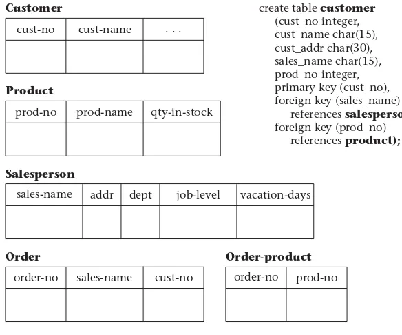
Step III Physical design
Step II(c) Transformation of the conceptual model to SQL tables
Step II(d) Normalization of SQL tables Customer
Product
prod-no prod-name qty-in-stock cust-no
sales-name
sales-name addr
addr dept
dept
job-level
job-level job-level vacation-days
vacation-days
Order-product
order-no prod-no
Order
order-no sales-name cust-no cust-name . . .
Salesperson
Decomposition of tables and removal of update anomalies
Indexing Clustering Partitioning Materialized views Denormalization
Salesperson Sales-vacations
create table customer
(cust_no integer, cust_name char(15), cust_addr char(30), sales_name char(15), prod_no integer, primary key (cust_no), foreign key (sales_name) references salesperson
foreign key (prod_no) references product);
FIGURE 1.2
consolidated into a single global view. View integration requires the use of ER semantic tools such as identifi cation of synonyms, aggregation, and generalization. In Figure 1.2 (step II(b)), two possible views of the product/ customer database are merged into a single global view based on common data for customer and order. View integration is also important for applica-tion integraapplica-tion.
c. Transformation of the conceptual data model to SQL tables. Based on a categorization of data modeling constructs and a set of mapping rules, each relationship and its associated entities are transformed into a set of DBMS-specifi c candidate relational tables. Redundant tables are eliminated as part of this process. In our example, the tables in step II(c) of Figure 1.2 are the result of transformation of the integrated ER model in step II(b). d. Normalization of tables. Functional dependencies (FDs) are derived from
the conceptual data model diagram and the semantics of data relationships in the requirements analysis. They represent the dependencies among data elements that are unique identifi ers (keys) of entities. Additional FDs that represent the dependencies among key and nonkey attributes within enti-ties can be derived from the requirements specifi cation. Candidate rela-tional tables associated with all derived FDs are normalized (i.e., modifi ed by decomposing or splitting tables into smaller tables) using standard tech-niques. Finally, redundancies in the data in normalized candidate tables are analyzed further for possible elimination, with the constraint that data integrity must be preserved. An example of normalization of the Sales-person table into the new Salesperson and Sales-vacations tables is shown in Figure 1.2 from step II(c) to step II(d).
We note here that database tool vendors tend to use the term logical model to refer to the conceptual data model, and they use the term physi-cal model to refer to the DBMS-specifi c implementation model (e.g., SQL tables). Note also that many conceptual data models are obtained not from scratch, but from the process of reverse engineering from an existing DBMS-specifi c schema (Silberschatz, Korth, & Sudarshan, 2002).
III. Physical design. The physical design step involves the selection of indexes (access methods), partitioning, and clustering of data. The logical design methodology in step II simplifi es the approach to designing large relational databases by reducing the number of data dependencies that need to be ana-lyzed. This is accomplished by inserting conceptual data modeling and integra-tion steps (II(a) and II(b) of Figure 1.2 ) into the tradiintegra-tional relaintegra-tional design approach. The objective of these steps is an accurate representation of reality. Data integrity is preserved through normalization of the candidate tables created when the conceptual data model is transformed into a relational model. The purpose of physical design is to optimize performance as closely as possible.
there are obvious, large gains to be made in effi ciency. This is called denor-malization . It consists of selecting dominant processes on the basis of high frequency, high volume, or explicit priority; defi ning simple extensions to tables that will improve query performance; evaluating total cost for query, update, and storage; and considering the side effects, such as possible loss of integrity. This is particularly important for Online Analytical Processing (OLAP) applications.
IV. Database implementation, monitoring, and modifi cation. Once the design is completed, the database can be created through implementation of the formal schema using the data defi nition language (DDL) of a DBMS. Then the data manipulation language (DML) can be used to query and update the database, as well as to set up indexes and establish constraints, such as refer-ential integrity. The language SQL contains both DDL and DML constructs; for example, the create table command represents DDL, and the select command represents DML.
As the database begins operation, monitoring indicates whether perfor-mance requirements are being met. If they are not being satisfi ed, modifi ca-tions should be made to improve performance. Other modifi caca-tions may be necessary when requirements change or when the end users ’ expectations increase with good performance. Thus, the life cycle continues with monitor-ing, redesign, and modifi cations.
1.3
CONCEPTUAL DATA MODELING
Conceptual data modeling is the driving component of logical database design. Let us take a look at how this component came about, and why it is important. Schema diagrams were formalized in the 1960s by Charles Bachman. He used rectangles to denote record types and directed arrows from one record type to another to denote a one-to-many relationship among instances of records of the two types. The ER approach for conceptual data modeling was fi rst presented in 1976 by Peter Chen. The Chen form of the ER model uses rectangles to specify entities, which are somewhat analogous to records. It also uses diamond-shaped objects to represent the various types of relationships, which are differentiated by numbers or letters placed on the lines connecting the diamonds to the rectangles.
The Unifi ed Modeling Language (UML) was introduced in 1997 by Grady Booch and James Rumbaugh and has become a standard graphical language for specifying and documenting large-scale software systems. The data modeling component of UML (now UML 2.0) has a great deal of similarity with the ER model, and will be presented in detail in Chapter 3 . We will use both the ER model and UML to illustrate the data modeling and logical database design examples.
approaches are most useful, is to capture real-world data requirements in a simple and meaningful way that is understandable by both the database designer and the end user. The end user is the person responsible for accessing the database and executing queries and updates through the use of DBMS software, and therefore has a vested interest in the database design process.
The ER model has two levels of defi nition — one that is quite simple and another that is considerably more complex. The simple level is the one used by most current design tools. It is quite helpful to the database designer who must com-municate with end users about their data requirements. At this level you simply describe, in diagram form, the entities, attributes, and relationships that occur in the system to be conceptualized, using semantics that are defi nable in a data dic-tionary. Specialized constructs, such as “ weak ” entities or mandatory/optional existence notation, are also usually included in the simple form. But very little else is included, to avoid cluttering up the ER diagram while the designer ’ s and end users ’ understandings of the model are being reconciled.
An example of a simple form of ER model using the Chen notation is shown in Figure 1.3 . In this example, we want to keep track of videotapes and customers in a video store. Videos and customers are represented as entities Video and Cus-tomer , and the relationship rents shows a many-to-many association between them. Both Video and Customer entities have a few attributes that describe their characteristics, and the relationship rents has an attribute due date that repre-sents the date that a particular video rented by a specifi c customer must be returned.
From the database practitioner ’ s standpoint, the simple form of the ER model (or UML) is the preferred form for both data modeling and end user verifi cation. It is easy to learn and applicable to a wide variety of design problems that might be encountered in industry and small businesses. As we will demonstrate, the simple form can be easily translated into SQL data defi nitions, and thus it has an immediate use as an aid for database implementation.
due-date cust-id
cust-name
N N
Customer Video
video-id
copy-no
title rents
FIGURE 1.3
The complex level of ER model defi nition includes concepts that go well beyond the simple model. It includes concepts from the semantic models of arti-fi cial intelligence and from competing conceptual data models. Data modeling at this level helps the database designer capture more semantics without having to resort to narrative explanations. It is also useful to the database application pro-grammer, because certain integrity constraints defi ned in the ER model relate directly to code — for example, code that checks range limits on data values and null values. However, such detail in very large data model diagrams actually detracts from end user understanding. Therefore, the simple level is recommended as the basic communication tool for database design verifi cation.
1.4
SUMMARY
Knowledge of data modeling and database design techniques is important for database practitioners and application developers. The database life cycle shows the steps needed in a methodical approach to designing a database, from logical design, which is independent of the system environment, to physical design, which is based on the details of the database management system chosen to implement the database. Among the variety of data modeling approaches, the ER and UML data models are arguably the most popular ones in use today, due to their simplicity and readability. A simple form of these models is used in most design tools; it is easy to learn and to apply to a variety of industrial and business applications. It is also a very useful tool for communicating with the end user about the conceptual model and for verifying the assumptions made in the mod-eling process. A more complex form, a superset of the simple form, is useful for the more experienced designer who wants to capture greater semantic detail in diagram form, while avoiding having to write long and tedious narrative to explain certain requirements and constraints.
1.5
LITERATURE SUMMARY
2
Entity – Relationship
Concepts
Until now we have dealt with databases made up of a number of distinct tables, without concerning ourselves very much with how the tables and their constitu-ent columns were originally generated. Logical database design , also known simply as database design or database modeling , studies basic properties and interrelationships among data items, with the aim of providing faithful representa-tions of such items in the basic data structures of a database. Databases with dif-ferent data models have difdif-ferent structures for representing data; in relational databases the fundamental structures for representing data are what we have been calling relational tables. We concentrate on relational databases in this chapter because design for the object-relational model is still in its infancy.
It is the responsibility of the database administrator (DBA) to perform this logical database design, assigning the related data items of the database to columns of tables in a manner that preserves desirable properties. The most important test of logical design is that the tables and attributes faithfully refl ect interrelationships among objects in the real world and that this remains true after all likely database updates in the future.
The DBA starts by studying some real-world enterprise, such as a wholesale order business, a company personnel offi ce, or a college registration department, whose operation needs to be supported on a computerized database system. Often working with someone who has great expertise about the details of the enterprise, the DBA comes up with a list of data items and underlying data objects that must be kept track of (in college student registration, this list might include student _ names , courses , course _ sections , class _ rooms , class _ periods , etc.), together with a number of rules, or constraints , concerning the interrelatedness of these data items. Typical rules for student registration are the following:
■ Every registered student has a unique student ID number (which we name sid ).
■ A classroom can house at most one course section for a given class period.
■ And so on.
From these data items and constraints, the DBA is expected to perform the logical design of the database. Two common techniques covered in this chapter are used to perform the task of database design. The fi rst is known as the
entity – relationship approach (or ER approach), and the second is the normaliza-tion approach. The ER approach attempts to provide a taxonomy of data items to allow a DBA to intuitively recognize different types of data classifi cation objects (entities, weak entities, attributes, relationships, etc.) to classify the listed data items and their relationships. After creating an ER diagram that illustrates these objects, a relatively straightforward procedure allows the DBA to translate the design into relational tables and integrity constraints in the database system. The normalization approach seems entirely different, and perhaps less dependent on intuition: all the data items are listed, and then all interrelatedness rules (of a recognized kind, known as dependencies ) are identifi ed. Design starts with the assumption that all data items are placed in a single huge table and then proceeds to break down the table into smaller tables. In the resulting set of tables, joins are needed to retrieve the original relationships. Both the ER modeling approach and the normalization approach are best applied by a DBA with a developed intuition about data relationships in the real world and about the way those relationships are ultimately modeled as relational tables. The two approaches tend to lead to identical relational table designs and in fact reinforce one another in providing the needed intuition. We will not attempt to discriminate between the two in terms of which is more applicable.
One of the major features of logical database design is the emphasis it places on rules of interrelationships between data items. The naive user often sees a relational table as made up of a set of descriptive columns, one column much like another. But this is far from accurate, because there are rules that limit possible relationships between values in the columns. For example, a customers table, conceived as a relation, is a subset of the Cartesian product of four domains, CP = CID × CNAME × CITY × DISCNT . However, in any legal customers table, two rows with the same customer ID ( cid ) value cannot exist because cid is a unique identifi er for a customers row. Here is a perfect example of the kind of rule we wish to take into account in our logical database design. A faithful table represen-tation enforces such a requirement by specifying that the cid column is a candi-date key or the primary key for the customers table. A candidate key is a designated set of columns in a table such that two table rows can never be alike in all these column values, and where no smaller subset of the key columns has this property. A primary key is a candidate key that has been chosen by the DBA for external reference from other tables to unique rows in the table.
The fact that the ssn column is declared as not null unique in a Create Table statement simply means that in any permitted customers content, two rows cannot have the same ssn value, and thus it is a candidate key. When cid is declared as a primary key in the Create Table statement, this is a more far-reaching statement, making cid the identifi er of customers rows that might be used by other tables. Following either of the table defi nitions of 2.1, a later SQL Insert or Update statement that would duplicate a cid value or ssn value on two rows of the customers table is illegal and has no effect. Thus, a faithful representation of the table key is maintained by the database system.
Also a number of other clauses of the Create Table statement serve a comparable purpose of limiting possible table content, and we refer to these as integrity con-straints for a table. The interrelationships between columns in relational tables must be understood at a reasonably deep level in order to properly appreciate some constraints. Although not all concepts of logical design can be faithfully represented in the SQL of today, SQL is moving in the direction of modeling more and more such concepts. In any event, many of the ideas of logical design can be useful as an aid to systematic database defi nition even in the absence of direct system support.
In the following sections, we fi rst introduce a number of defi nitions of the ER model. The process of normalization is introduced after some ER intuition has been developed.
2.1
INTRODUCTION TO ER CONCEPTS
The ER approach attempts to defi ne a number of data classifi cation objects; the database designer is then expected to classify data items by intuitive recognition as belonging in some known classifi cation. Three fundamental data classifi cation objects introduced in this section are entities, attributes, and relationships.
2.1.1
Entities, Attributes, and Simple ER Diagrams
We begin with a defi nition of the concept of entity .
Defi nition: Entity. An entity is a collection of distinguishable real-world objects with common properties.
For example, in a college registration database we might have the following entities: Students , Instructors , Class _ rooms , Courses , Course _ sections , FIGURE 2.1
SQL declaration of customers table with primary key cid and candidate key ssn .
Class _ periods , and so on. (Note that entity names are capitalized.) Clearly the set of classrooms in a college fi ts our defi nition of an entity: individual classrooms in the entity Class _ rooms are distinguishable (by location — i.e., room number) and have other common properties such as seating capacity (not common values, but a common property). Class _ periods is a somewhat surprising entity — is “ MWF from 2:00 to 3:00 PM ” a real-world object? However, the test here is that the registration process deals with these class periods as if they were objects, assigning class periods in student schedules in the same sense that rooms are assigned.
To give examples of entities that we have worked with a good deal in the CAP database, we have Customers , Agents , and Products . ( Orders is also an entity, but there is some possibility for confusion in this, and we discuss it a bit later.) There is a foreshadowing here of entities being mapped to relational tables. An entity such as Customers is usually mapped to an actual table, and each row of the table corresponds to one of the distinguishable real-world objects that make up the entity, called an entity instance , or sometimes an entity occurrence.
Note that we do not yet have a name for the properties by which we tell one entity occurrence from another, the analog to column values to distinguish rows in a relational table. For now we simply refer to entity instances as being distin-guishable, in the same sense that we would think of the classrooms in a college as being distinguishable, without needing to understand the room-labeling scheme used. In what follows we always write an entity name with an initial capital letter, but the name becomes all lowercase when the entity is mapped to a relational table in SQL.
We have chosen an unusual notation by assigning plural entity names: Students , Instructors , Class _ rooms , and so forth. More standard would be entities named Student , Instructor , and Class _ room . Our plural usage is chosen to emphasize the fact that each represents a set of real-world objects, usually containing multiple elements, and carries over to our plural table names (also somewhat unusual), which normally contain multiple rows. Entities are repre-sented by rectangles in ER diagrams, as you can see by looking at Figure 2.2 .
Note that some other authors use the terminology entity set or entity type in referring to what we call an entity. Then to these authors, an entity is what we would refer to as an entity instance. We have also noticed occasional ambiguity within a specifi c author ’ s writing, sometimes referring to an entity set and some-times to an entity; we assume that the object that is represented by a rectangle in an ER diagram is an entity, a collection of real-world objects, and authors who identify such rectangles in the same way agree with our defi nition. It is unfortunate that such ambiguity exists, but our notation will be consistent in what follows.
In mathematical discussion, for purposes of defi nition, we usually represent an entity by a single capital letter, possibly subscripted where several exist (e.g., E, E 1 , E 2 , etc.). An entity E is made up of a set of real-world objects, which we
above, each distinct representative e i of an entity E is called an entity instance or
an entity occurrence.
Defi nition: Attribute. An attribute is a data item that describes a property of an entity or a relationship (defi ned below).
Recall from the defi nition of entity that all entity occurrences belonging to a given entity have common properties. In the ER model, these properties are known as attributes . As we will see, there is no confusion in terminology between an attribute in the ER model and an attribute or column name in the relational model, because when the ER design is translated into relational terms, the two correspond. A particular instance of an entity is said to have attribute values for all attributes describing the entity (a null value is possible). The reader should keep in mind that while we list distinct entity occurrences {e 1 , e 2 , . . . , e n } of the
entity E, we can ’ t actually tell the occurrences apart without reference to attribute values.
Each entity has an identifi er , an attribute, or set of attributes that takes on unique values for each entity instance; this is the analog of the relational concept of candidate key . For example, we defi ne an identifi er for the Customers entity to be the customer identifi er, cid . There might be more than one identifi er for a given entity, and when the DBA identifi es a single key attribute to be the univer-sal method of identifi cation for entity occurrences throughout the database, this is called a primary identifi er for the entity. Other attributes, such as city for Customers , are not identifi ers but descriptive attributes , known as descriptors . Most attributes take on simple values from a domain, as we have seen in the rela-tional model, but a composite attribute is a group of simple attributes that together describe a property. For example, the attribute student _ names for the Students entity might be composed of the simple attributes lname , fname , and midinitial . Note that an identifi er for an entity is allowed to contain an attribute of composite type. Finally, we defi ne a multivalued attribute to be one that can take on multiple values for a single entity instance. For example, the Employees entity might have an attached multivalued attribute named hobbies , which takes FIGURE 2.2
Example of ER diagrams with entities and attributes.
Employees
city state zipcode
hobbies eid
staddress midinitial
sid
student_name Students
emp_address lname
on multiple values provided by the employee asked to list any hobbies or interests. One employee might have several hobbies, so this is a multivalued attribute.
As mentioned earlier, ER diagrams represent entities as rectangles. Figure 2.2 shows two simple ER diagrams. Simple, single-valued attributes are represented by ovals, attached by a straight line to the entity. A composite attribute is also in an oval attached directly to the entity, while the simple attributes that make up the composite are attached to the composite oval. A multivalued attribute is attached by a double line, rather than a single line, to the entity it describes. The primary identifi er attribute is underlined.
2.1.2
Transforming Entities and Attributes to Relations
Our ultimate aim is to transform the ER design into a set of defi nitions for relational tables in a computerized database, which we do through a set of transformation rules.
Transformation Rule 1. Each entity in an ER diagram is mapped to a single table in a relational database; the table is named after the entity. The table ’ s columns represent all the single-valued simple attributes attached to the entity (possibly through a composite attribute, although a composite attribute itself does not become a column of the table). An identifi er for an entity is mapped to a can-didate key for the table, as illustrated in Example 2.1 , and a primary identifi er is mapped to a primary key. Note that the primary identifi er of an entity might be a composite attribute, which therefore translates to a set of attributes in the relational table mapping. Entity occurrences are mapped to the table ’ s rows. ■
EXAMPLE 2.1
Here are the two tables, with one example row fi lled in, mapped from the Students and Employees entities in the ER diagrams of Figure 2.2 . The primary key is underlined.
students
sid lname fname Midinitial
1134 Smith John L.
. . . . . . . . . . . .
employees
eid staddress city state zipcode
197 7 Beacon St Boston MA 02122
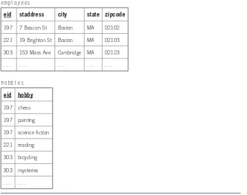
Transformation Rule 2. Given an entity E with primary identifi er p , a multivalued attributed attached to E in an ER diagram is mapped to a table of its own; the table is named after the plural multivalued attribute. The columns of this new table are named after p and a (either p or a might consist of several attributes), and rows of the table correspond to ( p, a ) value pairs, representing all pairings of attribute values of a associated with entity occurrences in E. The primary
key attribute for this table is the set of columns in p and a . ■
EXAMPLE 2.2
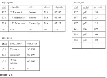
Here is an example database of two tables refl ecting the ER diagram for the Employees entity and the attached multivalued attribute, hobbies , of Figure 2.2 .
employees
eid staddress city state zipcode
197 7 Beacon St Boston MA 02102
221 19 Brighton St Boston MA 02103
303 153 Mass Ave Cambridge MA 02123
. . . . . . . . . . . . . . .
hobbies
eid hobby
197 chess
197 painting
197 science fi ction
221 reading
303 bicycling
303 mysteries
. . . . . .
2.1.3
Relationships among Entities
A particular occurrence of a relationship, corresponding to a tuple of entity occur-rences (e 1 , e 2 , . . . , e n ), where e i is an instance of E i in the ordered list of the
defi nition, is called a relationship occurrence or relationship instance . The number of entities m in the defi ning list is called the degree of the relationship. A relationship between two entities is known as a binary relationship . For example, we defi ne teaches to be a binary relationship between Instructors and Course _ sections . We indicate that a relationship instance exists by saying that a particular instructor teaches a specifi c course section. Another example of a relationship is works _ on , defi ned to relate the two entities Employees and Projects in a large company: Employees works _ on Projects .
A relationship can also have attached attributes. The relationship works _ on might have the attribute percent , indicating the percent of work time during each week that the employee is assigned to work on each specifi c project (see Figure 2.3 ). Note that this percent attribute attached to the works _ on relationship would be multivalued if attached to either entity Employees or Projects ; the percent attribute is only meaningful in describing a specifi c employee – project pair, and it is therefore a natural attribute of the binary relationship works _ on .
A binary relationship that relates an entity to itself (a subset of E 1 × E 1 ) is called
a ring , or sometimes a recursive relationship . For example, the Employees entity is related to itself through the relationship manages , where we say that one employee manages another. Relationships are represented by diamonds in an ER diagram, with connecting lines to the entities they relate. In the case of a ring, the connecting lines are often labeled with the names of the roles played by the entity instances involved. In Figure 2.3 the two named roles are manager _ of and reports _ to .
Note that we often leave out attributes in an ER diagram to concentrate on relationships between entities without losing our concentration in excessive detail.
FIGURE 2.3
Examples of ER diagrams with relationships.
Employees works_on Projects
percent
Instructors teaches Course_sections
Employees manages
percent
EXAMPLE 2.3
The orders Table in CAP Does Not Represent a Relationship
Per the relationship defi nition, the orders table in the CAP database is not a relationship between Customers , Agents , and Products . This is because (cid, aid, pid) triples in the rows of the orders table do not identify a subset of the Cartesian product, Customers
× Agents × Products , as required. Instead, some triples of (cid, aid, pid) values occur more than once, and no doubt clearly the designer ’ s intention, since the same customer can order the same product from the same agent on two different occasions. Instead of a relationship, the orders table represents an entity in its own right, with identifi er attribute ordno . This makes a good deal of sense, since we might commonly have reason to look up a row in the orders table for reasons unconnected to relating entity occurrences in Cus-tomers , Agents , and Products . For example, on request, we might need to check that a past order has been properly billed and shipped. Thus, the entity Orders occurrences are dealt with individually as objects in their own right.
Although the orders table doesn ’ t correspond directly to a relationship, it is clear that there are any number of possible relationships we could defi ne in terms of the orders table between the Customers , Agents , and Products entities.
EXAMPLE 2.4
Assume that we are performing a study in which we commonly need to know total sales aggregated (summed) from the orders table by customers , agents , and products for the current year. We might do this, for example, to study sales volume relationships between agents and customers , as well as between customers and products , and how those relationships are affected by geographic factors ( city values). However, as we begin to plan this application, we decide that it is too ineffi cient to always perform sums on the orders table to access the basic measures of our study, so we decide to create a new table called yearlies . We defi ne this new table with the following SQL commands:
create table yearlies (cid char(4). aid char(3). pid char(3).
totqty integer, totdoll float);
insert into yearlies
select cid, aid, pid, sum(qty), sum(dollars) from orders
group by cid, aid, pid;
Once we have the new yearlies table, the totals can be kept up to date by application logic: As each new order is entered, the relevant yearlies row should be updated as well. Now the yearlies table is a relationship, since the (cid, aid, pid) triples in the rows of the table identify a subset of the Cartesian product, Customers × Agents × Products ; that is to say, there are now no repeated triples in the yearlies table. Since these triples are unique, (cid, aid, pid) forms the primary key for the yearlies table.
of distinct binary relationships in an ER diagram, and this is a good idea if the replacement expresses true binary relationships for the system. Binary relation-ships are the ones that are familiar to most practitioners and are suffi cient for almost all applications. However, in some cases, a ternary relationship cannot be decomposed into expressive binary relationships. The yearlies relationship of Example 2.4 expresses customer-agent-product ordering patterns over a year, a ternary relationship that cannot be decomposed (exactly) into binary relation-ships. In converting an ER design to a relational one, a relationship is sometimes translated into a relational table, and sometimes not. (We will have more to say about this in the next section.) For example, the yearlies relationship (a ternary relationship) is translated into a relational table named yearlies . However, the manages relationship between Employees and Employees , shown in Figure 2.3 , does not translate into a table of its own. Instead, this relationship is usually trans-lated into a column in employees identifying the mgrid to whom the employee reports. This table is shown again in Figure 2.4 .
Note the surprising fact that mgrid is not considered an attribute of the Employees entity, although it exists as a column in the employees table. The mgrid column is what is known as a foreign key in the relational model, and it corre-sponds to the actual manages relationship in the ER diagram of Figure 2.3 . We deal more with this in the next section, after we have had an opportunity to consider some of the properties of relationships. To summarize this section, Figure 2.5(a) and (b) lists the concepts introduced up to now.
2.2
FURTHER DETAILS OF ER MODELING
Now that we ’ ve defi ned some fundamental means of classifi cation, let ’ s discuss properties of relationships in the ER method of database design.
FIGURE 2.4
A table representing an entity, Employees , and a ring (recursive relationship), manages .
employees
eid ename mgrid
FIGURE 2.5
Basic ER concepts: (a) entities and attributes, and (b) relationships.
Classification Description Example
Entity A collection of distinguishable real-world objects with common properties
Customers, Agents, Products, Employees
Attribute A data item that describes a property of an
entity or relationship See below
Descriptor Non-key attribute, describing an entity or relationship
city (for Customers), capacity
(for Class_rooms)
Composite attribute
A group of simple attributes that together
describe a property of an object emp_address (see Figure 2.2)
Multi-valued attribute
An entity attribute that takes on multiple values for a single entity instance
(a)
(b)
hobbies (see Figure 2.2)
Classification Description Example
Relationship Named set of m-tuples, identifies subset of the Cartesian product E1× E2× . . . × Em Binary
relationship
A relationship on two distinct entities teaches,works_on (see Figure 2.3)
Ring, recursive relationship
A relationship relating an entity to itself manages (see Figure 2.4)
Ternary relationship
A relationship on three distinct entities yearlies (see Example 2.4)
2.2.1
Cardinality of Entity Participation in a Relationship
Figure 2.6 illustrates the concepts of minimum and maximum cardinality with which an entity participates in a relationship. Figure 2.6(a), (b), and (c) represent entities E and F on the left and right, respectively, by two sets; elements of the two sets are connected by a line exactly when a relationship R relates the two entity occurrences represented. Thus, the connecting lines themselves represent instances of the relation R. Note that the diagrams of Figure 2.6 are not what we refer to as ER diagrams.
as the row content of a table can change, until some entity instances have differ-ent numbers of lines connected. On the other hand, the minimum and maximum cardinality properties of an entity are meant to represent rules laid down by the DBA for all time, rules that cannot be broken by normal database changes affect-ing the relationship. In Figure 2.6(a) , the DBA clearly permits both entity sets E and F to take part in relationship R with minimum cardinality 0; that is to say, the DBA does not require a connecting line for each entity instance, since some ele-ments of both sets have no lines connected to them. We symbolize this by writing min-card(E, R) = 0 and min-card(F, R) = 0. The maximum cardinality with which E and F take part in R is not obvious from Figure 2.6(a) , however. No entity instance has more than one line connected to it, but from an example as of a given moment we have no guarantee that the line connections won ’ t change in the future so that some entity instances will have more than one line connected. However, we will assume for purposes of simple explanation that the diagrams of this fi gure are meant to represent exactly the cardinalities intended by the DBA. Thus, since no entity instance of E and F in Figure 2.6(a) has more than one inci-dent connecting line, we record this fact using the notation max-card(E, R) = 1 and max-card(F, R) = 1.
In Figure 2.6(b) , assuming once again that this set of lines is representative of the designer ’ s intention, we can write min-card(E, R) = 0, since not every element of E is connected to a line, but min-card(F, R) = 1, since at least one line is con-nected to every element of F, and our assumption implies that this won ’ t change. We also write max-card(E, R) = N, where N means “ more than one ” ; this means that the designer does not intend to limit to one the number of lines connected to each entity instance of E. However, we write max-card(F, R) = 1, since every element of F has exactly one line leaving it. Note that the two meaningful values for min-card are 0 and 1 (where 0 is not really a limitation at all, but 1 stands for FIGURE 2.6
Examples of relationships R between two entities E and F.
E R F E R F E R F
(a) One-to-one relationship (b) Many-to-one relationship (c) Many-to-many relationship min-card(E, R) = 0 min-card(E, R) = 0 min-card(E, R) = 0 max-card(E, R) = 1 max-card(E, R) = N max-card(E, R) = N min-card(F, R) = 0 min-card(F, R) = 1 min-card(F, R) = 0 max-card(F, R) = 1 max-card(F, R) = 1 max-card(F, R) = N
the constraint “ at least one ” ), and the two meaningful values for max-card are 1 and N (N is not really a limitation, but 1 represents the constraint “ no more than one ” ). We don ’ t try to differentiate numbers other than 0, 1, and many. Since max-card(E, R) = N, there are multiple entity instances of F connected to one of E by the relationship. For this reason, F is called the “ many ” side and E is called the “ one ” side in this many-to-one relationship.
Note particularly that the “ many ” side in a many-to-one relationship is the side that has max-card value 1! In Figure 2.6(b) , the entity F corresponds to the “ many ” side of the many-to-one relationship, even though it has min-card(F, R) = max-card(F, R) = 1. As just explained, the “ one ” side of a many-to-one relationship is the side where some entity instances can participate in multiple relationship instances, “ shooting out multiple lines ” to connect to many entity instances on the “ many ” side! Phrased this way the terminology makes sense, but this seems to be an easy idea to forget, and forgetting it can lead to serious confusion.
In Figure 2.6(c) we have min-card(E, R) = 0, min-card(F, R) = 0, max-card(E, R) = N, and max-card(F, R) = N. The meaning of the terms used for the three diagrams — one-to-one relationship, many-to-one relationship, and many-to-many relationship — are defi ned later.
EXAMPLE 2.5
In the relationship teaches of Figure 2.3 , Instructors teaches Course _ sections , the DBA would probably want to make a rule that each course section needs to have at least one instructor assigned to teach it by writing min-card( Course _ sections , teaches ) = 1. However, we need to be careful in making such a rule, since it means that we will not be able to create a new course section, enter it in the database, assign it a room and a class period, and allow students to register for it, while putting off the decision of who is going to teach it. The DBA might also make the rule that at most one instructor can be assigned to teach a course section by writing max-card( Course _ sections , teaches ) = 1. On the other hand, if more than one instructor were allowed to share the teaching of a course section, the DBA would write max-card( Course _ sections , teaches ) = N. This is clearly a signifi cant difference. We probably don ’ t want to make the rule that every instructor teaches some course section (written as min-card( Instructors , teaches ) = 1), because an instructor might be on leave, so we settle on min-card( Instructors , teaches ) = 0. And in most universities the course load per instructor is greater than one in any given term, so we would set max-card( Instructors , teaches ) = N.
Defi nition. When an entity E takes part in a relationship R with min-card(E, R) = x (x is either 0 or 1) and max-card(E, R) = y (y is either 1 or N), then in the ER diagram the connecting line between E and R can be labeled with the ordered cardinality pair (x, y). We use a new notation to represent this minimum-maximum pair (x, y): card(E, R) = (x, y).
labeled with the pair (1, 1). In Figure 2.7 we repeat the ER diagrams of Figure 2.3 , with the addition of ordered pairs (x, y) labeling line connections, to show the minimum and maximum cardinalities for all ER pairs. The cardinality pair for the Instructors teaches Course _ sections diagram follows the discussion of Example 2.5 , and other diagrams are fi lled in with reasonable pair values. We make a number of decisions to arrive at the following rules: Every employee must work on at least one project (but may work on many); a project might have no employees assigned during some periods (waiting for staffi ng), and of course some projects will have a large number of employees working on them; an employee who acts in the manager _ of role (see discussion below) may be managing no other employees at a given time and still be called a manager; and an employee reports to at most one manager, but may report to none (this possibility exists because there must always be a highest-level employee in a hierarchy who has no manager).
In the Employees-manages diagram shown in Figure 2.7 , the normal notation, card(Employees , manages) , would be ambiguous. We say that there are two dif-ferent roles played by the Employees entity in the relationship: the manager _ of role and the reports _ to role. Each relationship instance in manages connects a
managed employee ( Employees instance in the reports _ to role) to a manager employee ( Employees instance in the manager _ of role). We use the cardinality notation with entities having parenthesized roles to remove ambiguity.
card(Employees(reports _ to). manages) = (0. 1) and
card(Employees(manager _ of). manages) = (0. N)
And from these cardinalities we see that an employee who acts in the manager _ of role may be managing no other employees at a given time and still be called a manager; and an employee reports to at most one manager, but may report to none (because of the highest-level employee in a hierarchy who has no manager — if it weren ’ t for that single person, we could give the label (1, 1) to the reports _ to branch of the Employees-manages edge).
FIGURE 2.7
An ER diagram with labels (x, y) on ER connections.
Employees works_on Projects
percent
Instructors teaches Course_sections
Employees manages
ename
reports_to manager_of
(0, 1) (1, 1)
(0, N)
(0, N) (0, N)
Defi nition. When an entity E takes part in a relationship R with max-card(E, R) = 1, then E is said to have single-valued participation in the relationship R. If max-card(E, R) = N, then E is said to be multivalued in this relationship. A binary relationship R between entities E and F is said to be many-to-many , or N-N, if both entities E and F are multi-valued in the relationship. If both E and F are single-valued, the relationship is said to be one-to-one , or 1-1. If E is single-valued and F is multivalued, or the reverse, the relationship is said to be many-to-one, or N-1. (We do not normally speak of a 1-N relationship as distinct from an N-1 relationship.)
2.2.2
One-to-One, Many-to-Many, and Many-to-One Relationships
Recall that the “ many ” side in a many-to-one relationship is the side that has single-valued participation. This might be better understood by considering the relationship in Figure 2.7 , Instructors teaches Course _ sections , where card (Course _ sections , teaches) = (1, 1), and the Course _ sections entity represents the “ many ” side of the relationship. This is because one instructor teaches “ many ” course sections, while the reverse is not true.
In the last defi nition, we see that the values max-card(E, R) and max-card(F, R) determine whether a binary relationship is many-to-many, many-to-one, or one-to-one. On the other hand, the values min-card(E, R) and min-card(F, R) are not mentioned, and they are said to be independent of these characterizations. In particular, the fact that min-card(F, R) = 1 in Figure 2.6(b) is independent of the fact that that fi gure represents a many-to-one relationship. If there were addi-tional elements in entity F that were not connected by any lines to elements in E (but all current connections remained the same), this would mean that min-card(F, R) = 0, but the change would not affect the fact that R is a many-to-one relation-ship. We would still see one element of E (the second from the top) related to two elements of F; in this case, the entity F is the “ many ” side of the relationship.
Although min-card(E, R) and min-card(F, R) have no bearing on whether a binary relationship R is many-to-many, many-to-one, or one-to-one, a different characterization of entity participation in a relationship is determined by these quantities.
Defi nition. When an entity E that participates in a relationship R has min-card(E, R) = 1, E is said to have mandatory participation in R, or is simply called mandatory in R. An entity E that is not mandatory in R is said to be optional, or to have optional participation.