Optimizing SVR using Local Best PSO for Software
Effort Estimation
Dinda Novitasari1, Imam Cholissodin2, Wayan Firdaus Mahmudy3
1,2,3Department of Informatics/ Computer Science, Brawijaya University, Indonesia 1[email protected], 2[email protected], 3[email protected]
Received 21 February 2016; received in revised form 18 March 2016; accepted 25 March 2016
Abstract. In the software industry world, it’s known to fulfill the tremendous demand. Therefore, estimating effort is needed to optimize the accuracy of the results, because it has the weakness in the personal analysis of experts who tend to be less objective. SVR is one of clever algorithm as machine learning methods that can be used. There are two problems when applying it; select features and find optimal parameter value. This paper proposed local best PSO-SVR to solve the problem. The result of experiment showed that the proposed model outperforms PSO-SVR and T-SVR in accuracy.
Keywords: Optimization, SVR, Optimal Parameter, Feature Selection, Local Best PSO, Software Effort Estimation
1 Introduction
[10]. The result, PSOs provide the excellent performance and effective in finding the most optimal solutions, rather than GA and others [11]. PSO improvements have been made to deal with premature convergence (local optimum), although the time it takes a little longer, but can still be tolerated and comparable to the best optimization results obtained, the name of the method is the Local best PSO utilize ring topology that illustrated in Fig. 1 [12],[13]. Thus, based on that reason, ring topology-based local best PSO-SVR is proposed in our paper.
Fig. 1. Ring topology
2 Method
2.1 Support Vector Regression
Given training data {xi,yi}, i = 1,...,l; xi∈ Rd; yi∈Rd where xi, yi is input (vector)
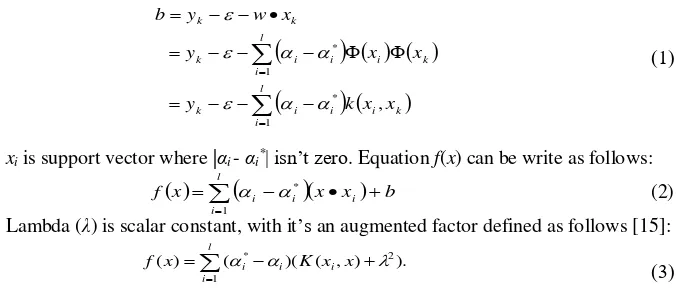
and output (scalar value as target). Other forms of alternative for bias to calculation f(x) is can be build solution like bias as follows [14]:
(1)
xi is support vector where |αi- αi*| isn’t zero. Equation f(x) can be write as follows:
(2) Lambda (λ) is scalar constant, with it’san augmented factor defined as follows [15]:
(3) 2.1.1 Sequential Algorithm for SVR
Vijayakumar has made tactical steps through the process of iteration to obtain the solution of optimization problems of any nature by way of a trade-off on the values of the weights xi, or called αi to make the results of the regression becomes closer to
actual value. The step by step as follows:
1. Set initialization
0
,
*
0
i
i
, and get Rij [R]ijK(xi,xj)
2 (4)
l i k i i i k l i k i i i k k k x x k y x x y x w y b 1 * 1 * , x
x x b fl
i
i i
i
1 * . ) ) , ( )( ( ) ( 1 2 *
l i i ii K x x
x
for i,j= 1,…,n
2. For each point, do looping, i=1 to n:
n j j j ij
i
i y R
E 1(* ) (5)
* min{max[ ( ), *], *}.
i i
i
i E C
(6)
min{max[ ( ), ], }.
i i i
i E C
(7)
* * *.
i i
i
(8)
iii. (9)
3. Repeat step 2 until met stop condition. Learning rate γ is computed from
diagonalofkernelmatrice
max) constant( rate
learning cLR (10)
2.2 Particle Swarm Optimization
This algorithm defined solution as each particle for any problem in dimension space j. Then, it’s extended by inertia weight to improves performance [16],[17]. Where xid, vid, yid is position, velocity, and personal best position of particle i, dimension d, and Ŷi is
best position found in the neighborhood Ni. Each particle’s neighborhood at ring
topology consists of itself and its immediate two neighbours using euclidean distance. (11)
(12)
vij(t), xij(t) is velocity and position of particle i in dimension j=1,...n at time t, c1 and c2
are cognitive and social components, r1j and r2j are rand[0,1]. yi and ŷ is obtained by
(13)
(14)
The inertia weight w, is follows equation
(15)
2.3.1 Binary PSO
Discrete feature space is set using binary PSO [18]. Each element of a particle can take on value 0 or 1. New velocity function is follows:
t
y t x
t
r c t x t y t r c t wv t v ij ij j ij ij j ij ij ˆ 1 2 2 1 1
t1 x
t v t1xi i i
t i y f t i x f t i x t i y f t i x f t i y t i y 1 if 1 1 if 1
t
Ni f
y
t
f
x
x Ni
yˆ 1 ˆ 1 min ,
maxmax max min max w iter iter iter w w
(16)
where vij(t) is obtained from (11). Using (16), the position update changes to
otherwise 0 1 if 11 r3 t sig v t
t
xij j ij (17)
where r3j(t) ~ U(0,1).
2.3 Local best PSO SVR Model 2.3.1 Particle Representation
In this paper, SVR nonlinear is defined by the parameter C , ε , λ, σ , cLR. The particle is consisted of six parts: C, ε, λ, σ, cLR (continuous-valued) and features mask (discrete-valued). Table 1 shows the representation of particle i with dimension nf+5
where nf is the number of features.
TABLE I. PARTICLE I IS CONSISTED OF SIX PARTS: C,Ε,Λ,Ε, CLR AND FEATURE MASK
Continuous-valued Discrete-valued
C ε λ Σ cLR Feature mask
Xi,1 Xi,2 Xi,3 Xi,4 Xi,5 Xi,6, Xi,7 ,...,Xi,nf
2.3.2 Objective Function
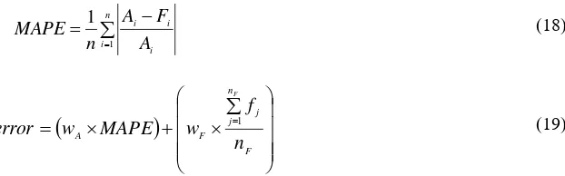
Objective function is used to measure how optimal the generated solution. There are two types of objective function: fitness and cost. The greater fitness value produced better solution. The lesser cost value produced better solution. In this paper, cost-typed is used as objective function because the purpose of this algorithm is to minimize the error. To design cost function, prediction accuracy and number of selected features are used as criteria. Thus, the particle with high prediction accuracy and small number of features produces a low prediction error with set weights value WA = 95% and WF
=5% [7]. n i i i i A F A n MAPE 1 1 (18)
F n j j F A n f w MAPE w error F 1 (19)where n is number of data, Ai is actual value and Fi is prediction value for data, fj is
value of feature mask.
ij
v t2.3.3 Local Best PSO SVR Algoritm
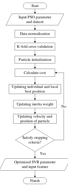
This paper proposed local best PSO-SVR algorithm to optimize SVR parameter and input feature mask simultaneously. Fig. 2 illustrates local best PSO-SVR algorithm. Details of algorithm are described as follows:
Start
Input PSO parameter and dataset
Optimized SVR parameter and input feature
Finish Updating inertia weight
Data normalization
K-fold cross validation
Particle initialization
Calculate cost
Updating individual and local best position
Updating velocity and position of particle
Satisfy stopping criteria?
Yes
No
Fig. 2. Flowchart of local best PSO-SVR
1. Normalizing data using
min max
min
x x
x x xn
(20)
where x is the original data from dataset, xmin and xmax is the minimum and
maximum value of original data, and xn is normalized value.
2. Dividing data into k to determine training and testing data. 3. Initializing a population of particle.
6. Updating inertia weight.
7. Updating velocity and position of each particle.
8. If stopping criteria is satisfied, and then end iteration. If not, repeat step 2. In this paper, stopping criteria is a given number of iterations.
3 Application of Local Best PSO-SVR in Software Effort
Estimation
3.1 Experimental settings
This study simulated 3 algorithms: local best PSO SVR, PSO SVR and T-SVR programmed using C#. For local best SVR simulation, we use the same parameters and dataset that is obtained from [19]. For software effort estimation, the inputs of SVR are Desharnais dataset [20]. The Desharnais dataset consists of 81 software projects are described by 11 variables, 9 independent variables and 2 dependent variables. For the experiment, we decide to use 77 projects due to incomplete provided features and 7 independent variables (TeamExp, ManagerExp, Transactions, Entities, PointsAdjust,
Envergure, and PointsNonAdjust) and 1 dependent variable (Effort). The PSO
parameters were set as in Table 2.
TABLE II. PSO PARAMETER SETTINGS
Number of fold Population of particles
Number of iterations Inertia weight(wmax, wmin) Acceleration coefficient(c1, c2)
Parameter searching space
10 15 40 (0,6, 0,2)
(1, 1,5)
C (0,1-1500), ε (0,001-0,009), σ (0,1-4), λ(0,01-3), cLR (0,01-1,75)
3.2 Experimental result
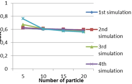
Fig. 3 illustrates the correlation between optimal cost and number of particle in 5 simulations. It showed that optimal cost is decreased while number of particle is being increased. From this chart, we can conclude that the more number of particles can provide more candidate solution so model can have more chance to select optimal solution. However, computing time is also increased because model spent much time to find solution among many particles and it is illustrated by Fig. 4. It happened because model must perform solution searching in many particles and it compromised computing time. In the experiment, we discovered that 20 particles could obtain the
Fig. 3. Comparison of number of particle
Fig. 4. Comparison of computing time
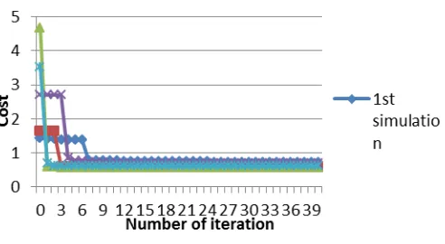
Fig. 5 illustrates the correlation between optimal cost and number of iteration in 5 simulations. It showed that optimal cost is decreased while number of iteration is being increased. For the example, in 4th simulation, optimal cost remained steady until 4th
iteration and move down until 8th iteration. From 8th iteration until 40th iteration,
Fig. 5. Convergence during process
Table 3 showed the comparison of the experiment results. The experiments showed that the proposed model outperforms T-SVR and PSO-SVR in optimizing SVR. Local best PSO SVR obtained lowest error among three models. It is observed that PSO-SVR spent less computing time because of fast convergence. Local best PSO-PSO-SVR model has slow convergence because it finds optimal solution in its neighborhood.
TABLE III. COMPARISON OF PREDICTION RESULTS
Model Time (ms)
Optimal (C, ε, σ,
cLR, λ)
Selected features Error
Local best PSO SVR
91.638 0,1000, 0,0063, 0,2536, 0,0100, 0,0100
2 (Entities and
Envergure)
0,5161
PSO-SVR
62.610 1500, 0,09, 0,1, 0,01, 3
2 (PointsAdjust and
Envergure)
0,5819
T-SVR 677.867 1055,3338, 0,0686, 0,1557, 0,1514, 0,2242
4 (TeamExp,
ManagerExp, Entities,
and PointsAdjust)
0,6086
4 Conclusion
software effort estimation problem. Hybridizing with other heuristic algorithms such as simulated annealing becomes an option to improve the performance of PSO [19][21].
References
[1] T. Standish Group, “Chaos Manifesto 2013 Think Big, Act Small,” 2013.
[2] R. Agarwal, M. Kumar, Yogesh, S. Mallick, R. M. Bharadwaj, and D. Anantwar,
“Estimating Software Projects,” ACM SIGSOFT Software Engineering Notes, vol. 26, no.
4, pp. 60–67, 2001.
[3] D. Zhang and J. J. Tsai, “Machine Learning and Software Engineering,” Software Quality
Journal, vol. 11, no. 2, pp. 87–119, 2003.
[4] K. Srinivasan and D. Fisher, “Machine Learning Approaches to Estimating Software
Development Effort,” IEEE Transactions on Software Engineering, vol. 21, no. 2, pp.
126–137, 1995.
[5] V. N. Vapnik, “An Overview of Statistical Learning Theory,” IEEE Transactions on
Neural Networks, vol. 10, no. 5, pp. 988–999, 1999.
[6] H. Frohlich, O. Chapelle, and B. Scholkopf, “Feature Selection for Support Vector
Machines by Means of Genetic Algorithm,” in Proceedings. 15th IEEE International
Conference on Tools with Artificial Intelligence, 2003, pp. 142–148.
[7] Y. Guo, “An Integrated PSO for Parameter Determination and Feature Selection of SVR
and Its Application in STLF,” in Proceedings of the Eighth International Conference on
Machine Learning and Cybernetics, Baoding, 12-15 July 2009, 2009, no. July, pp. 12–15.
[8] W. Wang, Z. Xu, W. Lu, and X. Zhang, “Determination of The Spread Parameter in the
Gaussian Kernel For Classification and Regression,” Neurocomputing, vol. 55, pp. 643–
663, 2003.
[9] P. Braga, A. Oliveira, and S. Meira, “A GA-based Feature Selection and Parameters
Optimization for Support Vector Regression Applied to Software Effort Estimation,” in
Proceedings of the 2008 ACM Symposium on Applied Computing, 2008, pp. 1788–1792.
[10] G. Hu, L. Hu, H. Li, K. Li, and W. Liu, “Grid Resources Prediction With Support Vector
Regression and Particle Swarm Optimization,” 3rd International Joint Conference on
Computational Sciences and Optimization, CSO 2010: Theoretical Development and Engineering Practice, vol. 1, pp. 417–422, 2010.
[11] M. Jiang, S. Jiang, L. Zhu, Y. Wang, W. Huang, and H. Zhang, “Study on Parameter
Optimization for Support Vector Regression in Solving the Inverse ECG Problem,”
Computational and Mathematical Methods in Medicine, vol. 2013, pp. 1–9, 2013.
[12] A. P. Engelbrecht, Computational Intelligence: An Introduction, 2nd ed. West Sussex: John Wiley & Sons Ltd, 2007.
[13] R. Mendes, J. Kennedy, and J. Neves, “The Fully Informed Particle Swarm: Simpler,
Maybe better,” IEEE Transactions on Evolutionary Computation, vol. 8, no. 3, pp. 204– 210, 2004.
[14] A. J. Smola and B. Scholkopf, “A Tutorial on Support Vector Regression,” Statistics and
Computing, vol. 14, no. 3, pp. 199–222, 2004.
[15] S. Vijayakumar and S. Wu, “Sequential Support Vector Classifiers and Regression,” in
Proceedings of International Conference on Soft Computing (SOCO ‘99), 1999, vol. 619,
[16] J. Kennedy and R. Eberhart, “Particle Swarm Optimization,” in Neural Networks, 1995.
Proceedings., IEEE International Conference on, 1995, vol. 4, pp. 1942–1948.
[17] Y. Shi and R. Eberhart, “A Modified Particle Swarm Optimizer,” in 1998 IEEE
International Conference on Evolutionary Computation Proceedings. IEEE World Congress on Computational Intelligence (Cat. No.98TH8360), 1998, pp. 69–73.
[18] J. Kennedy and R. C. Eberhart, “A discrete binary version of the particle swarm
algorithm,” in Proceedings of the World Miulticonference on Systemics, Cybernetics and Informatics, 1997, pp. 4104–4109.
[19] D. Novitasari, I. Cholissodin, and W. F. Mahmudy, “Hybridizing PSO with SA for Optimizing SVR Applied to Software Effort Estimation”, Telkomnika (Telecommunication
Computing Electronics and Control), 2015, vol. 14, no. 1, pp. 245-253.
[20] J. Sayyad Shirabad and T. J. Menzies, “The PROMISE Repository of Software
Engineering Databases,” School of Information Technology and Engineering, University
of Ottawa, Canada, 2005. [Online]. Available:
http://promise.site.uottawa.ca/SERepository. [Accessed: 05-Mar-2015].