Pharmaceutical and Medical Device Validation by Experimental Design

(1)

(2)

P

harmaceutical

and

m

edical

d

evice

v

alidation

by

(3)

(4)

Edited by

lynn d. torbeck

Torbeck & Associates, Inc.

Evanston, Illinois, USA

P

harmaceutical

and

m

edical

d

evice

v

alidation

by

(5)

New York, NY 10017

Printed in the United States of America on acid-free paper 10 9 8 7 6 5 4 3 2 1

International Standard Book Number-10: 1-4200-5569-0 (Hardcover) International Standard Book Number-13: 978-1-4200-5569-6 (Hardcover)

This book contains information obtained from authentic and highly regarded sources. Reprinted material is quoted with permission, and sources are indicated. A wide variety of references are listed. Reasonable efforts have been made to publish reliable data and information, but the author and the publisher cannot assume responsibility for the validity of all materials or for the consequence of their use.

No part of this book may be reprinted, reproduced, transmitted, or utilized in any form by any electronic, mechanical, or other means, now known or hereafter invented, including photocopying, microfilming, and recording, or in any information storage or retrieval system, without written permission from the publishers.

For permission to photocopy or use material electronically from this work, please access www.copyright.com (http://www.copyright.com/) or contact the Copyright Clearance Center, Inc. (CCC) 222 Rosewood Drive, Danvers, MA 01923, 978-750-8400. CCC is a not-for-profit organization that provides licenses and registration for a variety of users. For organizations that have been granted a photocopy license by the CCC, a separate system of payment has been arranged.

Trademark Notice: Product or corporate names may be trademarks or registered trademarks, and are used only for identification and explanation without intent to infringe.

Library of Congress Cataloging-in-Publication Data Pharmaceutical and medical device validation by experimental design / edited by Lynn D. Torbeck.

p. ; cm.

Includes bibliographical references and index. ISBN-13: 978-1-4200-5569-6 (hb : alk. paper)

ISBN-10: 1-4200-5569-0 (hb : alk. paper) 1. Pharmaceutical technology– Validity–Research–Methodology. 2. Experimental design.

I. Torbeck, Lynn D.

[DNLM: 1. Technology, Pharmaceutical–methods. 2. Multivariate Analysis. 3. Quality Control. 4. Reproducibility of Results. 5. Research Design. 6. Technology, Pharmaceutical–standards. QV 778 P5353995 2007]

RS192.P468 2007

615’.19–dc22 2007001418

Visit the Informa Web site at www.informa.com

(6)

Foreword

Imagine the following scenario: you have a seemingly impossible quality problem to solve. A new lyophilized product your com-pany is about to launch is apparently unstable at commercial scale. Management is breathing down your neck for an immedi-ate solution, since the research and development scale-up data indicated the formulation is stable. A crisis team was formed and has been working on a solution for almost six months.

Seeing the difficulty, a colleague suggests a different approach to looking at the problem, calling together a sub-team of four people that are the most knowledgeable about the production process. They use a few simple tools and deter-mine the most probable cause of the problem in a couple of hours using existing data. The resulting action plan corrects the problem, stable lyophilized lots are produced, and the product is launched on schedule. Does this sound too good to be true?

Fortunately, for those facing similar seemingly insupera-ble proinsupera-blems, the story is actually true. Not only is this specific story true, but also there are many more like it. Virtually every major biopharmaceutical company in the world has its own case study. These solutions were achieved thanks to a few simple process analysis tools and a systematic structured approach to visualizing data-rich experiments.

(7)

How do I know they work? Because I have personally used them, I have taught people to use them, and I have seen the results myself first hand.

Read this book. Buy copies for the people in your com-pany who work on difficult problems and train them in the methodology. Use the techniques to help find your own solu-tions to nearly impossible problems. Do not miss a chance to use the most powerful toolkit I have seen used in my 35 years in the industry. If you do not use these tools, you are also missing the opportunity to bring robust life saving therapeu-tics, as quickly as possible, to the people we really work for— the patients and their families.

THE APPROACH

DOE is an acronym for design of experiments, also called experimental design or multifactor experiments. These exper-imental approaches provide rich veins of data that can be mined for information that cannot be found any other way.

The reason for design in the description is that DOE experiments must be scientifically sound and statistically valid, especially for use in the highly regulated biopharma-ceutical industry. Scientific soundness is the cornerstone of the scientific peer review process, and (read world regulatory authority) Food and Drug Administration review and approval of such studies in support of product license approval. Statistical validity is necessary to ensure the integrity of the experiments and to appropriately interpret the significance of the data. In real terms, these are the same science and sta-tistics that are applied to clinical trials; now the application is being extended to production process monitoring, quality control testing, validation and process analytical technology or PAT. The DOE concepts are also valuable tools capable of being used to exploit existing data and help solve seemingly impossible product quality problems.

(8)

in order to explain the individual effect on product quality. By contrast, the design of experiments trials are carefully worked out to assess many possible factors (time, temperature, and pH) at various levels (one hour vs. two hours at 25°C vs. 30°C at pH 6.5 vs. pH 7.5) to determine which one, or combination, has the greatest effect on the product’s quality characteristics, such as yield, impurities, and viral reduction. DOE measures not only the single factor effects, but also the cumulative and interaction effects of all the factors investigated on product quality. Most important is the fact that DOE is the only way to see interaction effects; one factor at a time experiments give you just that, one effect for each factor.

INTERACTION EFFECTS

DOE is the only technique that enables scientists and manag-ers to find, see, and use interaction effects that can improve product quality and yield or help set process boundaries to prevent failure. The well entrenched views that only one factor at a time can be studied and the widely held management maxim that “if it ain’t broke, don’t fix it” are not only wrong but, in some cases, dangerous; a process can drift into failure, or periodically have an “unexplainable” failure, due to interac-tion effects. DOE permits scientists to conduct small scale, low cost process improvement experiments to model large scale, “unbroken” commercial processes without endangering current production runs and product supply. These same experiments can also generate data that drives continuous process improvement (read “make more profitable”) of a pro-cess that “ain’t broke.”

LEAST COST/FASTEST ROUTE

(9)

are usually conducted using a small scale process simula-tion—a much less expensive approach than tying up the pro-duction line. Third, the scale and cost of down-sized runs permits a relatively larger number of runs in a relatively short period of time. The resulting body of data provides a roadmap for process improvements that can be verified by additional small scale or scaled up experiments prior to full scale transi-tion that meets ongoing productransi-tion requirements.

VALIDATION

DOE’s data will define critical process parameters for valida-tion. The results of designed experiments are the identifica-tion of the individual parameters and those parameter interactions that have the most effect on product quality and yield. These are the critical process parameters that need to be assessed during process validation. Just as important, DOE identifies those parameters that do not impact product quality. These do not need to be validated but rather moni-tored and controlled within their defined process ranges. The savings of validating the DOE defined critical process param-eters versus validating “everything we think may be critical” is substantial in time, monetary, and human resource terms. Furthermore, given the scientific soundness and statistical validity of DOE results, processes validated using properly applied DOE principles are nearly bullet proof with the world’s regulatory agencies.

SUMMARY

(10)

provides data quicker than single factor at a time experiments. The proven statistical validity of the DOE technique guaran-tees accurate analysis of the data and valuable information for management to turn data analysis and interpretation into action.

Ronald C. Branning Genentech, Inc. South San Francisco, California, U.S.A.

(11)

(12)

Preface

Designed experiments were shown to be useful for validation almost 30 years ago. The famous chemist/statistician, W. J. Youden, illustrated the use of Plackett–Burman designs for ruggedness testing in the 1975 book, Statistical Manual of the Association of Official Analytical Chemists (1). In that short introduction, he noted that “… if the program is carefully laid out, a surprisingly small amount of work suffices.” The exam-ple given showed seven factors varied in eight runs. Each of the seven factors is estimated using all eight data values. This is the equivalent of having 56 data points, but only spending the money to buy eight. This efficiency is very attractive to laboratory managers who are charged with validating many analytical methods in a short time. Note that ruggedness test-ing is still required today by the Food and Drug Administration in the 1987 Guideline for Submitting Samples and Analytical Data for Method Validation (2).

This editor gave his first talk on using designed experi-ments in 1978 in response to the then draft Current Good Manufacturing Practices. In 1984, Chao, St. Forbes, Johnson, and von Doehren (3) gave an example of granulation valida-tion using a 23_{full factorial. Since then, there have been many} journal articles and conference talks showing the application

(13)

of designed experiments to validation. A recent addition is the text by Lewis et al., Pharmaceutical Experimental Design (4).

Yet, for all of the dispersed information and examples, there still is unease in the pharmaceutical industry about using designed experiments in general or for validation spe-cifically. Typical questions include, “What will the Food and Drug Administration say if I use a designed experiment for validation?” or “Won’t that take a lot longer and cost a lot more money?” In answer to the first question, the Food and Drug Administration requires the industry to use carefully designed experiments in clinical and animal studies. The well-regarded double blind clinical trial is a designed experiment. These are usually done exa ctly by the book. It is hard to see the Food and Drug Administration objecting to the use of designed experiments in validation when it is required in other areas. Further, in 1985, Ed Fry, while with the Food and Drug Administration, said in his excellent article “Then, the proc-esses that cause variability … must be identified. Experi ments are conducted (that is validation runs) to ensure that factors that would cause variability, are under control …” (5).

This book is the answer to the second question. Designed experiments are the most scientific, the most efficient, and the most cost effective way we know how to collect data. Designed experiments need not be complicated or statistically complex. Realistic case studies and examples illustrate the use of design of experiments for validation. The use of graphics illustrate the designs and results. Formulas are minimized and used only where necessary. Where possible, a step-by-step approach or procedure is given. Detailed protocols and reports with real-istic data are given where appropriate. This book succeeds if the reader feels that it is obvious that design of experiments is the most logical and rational approach to use.

A variety of examples and case studies are given to show the wide range of application. Assay and bioassay validation, process and equipment validation, etc. Not all cases are “end point” validation, but are further up-stream, and part of the life cycle validation discussed by Chapman (6).

(14)

chapters that seem most applicable and interesting. The text is intended to be a learn-by-doing-by-example. Find an exam-ple close to a intended project and mimic the approach.

It is hoped by the authors and the editor that this text will encourage people to use designed experiments for validation and learn first hand the benefits.

Lynn D. Torbeck

REFERENCES

1. Youden WJ. Statistical Manual of the Association of Official Analytical Chemists. Arlington, VA: AOAC, 1975.

2. FDA, Guideline for Submitting Samples and Analytical Data for Method Validation, Rockville, Maryland, 1987.

3. Chao A, Forbes S, Johnson, R, von Doehren P. Prospective proc-ess validation. In: Loftus B, Nash R, eds. Pharmaceutical Procproc-ess Validation. New York: Marcel Dekker, 1984:125–148.

4. Lewis G, Mathieu D, Phan-Tan-Luu R. Pharmaceutical Experimental Design. New York: Marcel Dekker, 1999.

5. Fry E. The FDA’s viewpoint. Drug and Cosmetic Industry 1985; 137(1):46–51.

6. Chapman K. A history of validation in the United States: part 1. Pharmaceutical Technology October 1991:82–96.

(15)

(16)

Contributors

Ronald C. Branning Genentech, Inc., South San Francisco, California, U.S.A.

Robert F. Dillard Biostatistics and Data Management, Takeda Pharmaceuticals North America, Inc., Lincolnshire, Illinois, U.S.A.

T. Lynn Eudey Department of Statistics, California State University East Bay, Hayward, California, U.S.A.

Jeffrey T. Field J. T. Field Consulting Services, LLC, Woodbury, Connecticut, U.S.A.

Sourav Kundu Technical Operations, Aventis Behring, Bradley, Illinois, U.S.A.

David M. Lansky Lansky Consulting, LLC, d/b/a Precision Bioassay, Burlington, Vermont, U.S.A.

Thomas D. Murphy T. D. Murphy Statistical Consulting, LLC, Morristown, New Jersey, U.S.A.

Daniel R. Pilipauskas Global Manufacturing Services, Pfizer, Inc., New York, New York, U.S.A.

(19)

Wayne A. Taylor Taylor Enterprises, Inc., Libertyville, Illinois, U.S.A.

(20)

1

Designing Experiments for

Validation of Quantitative Methods

T. LYNN EUDEY

Department of Statistics California State University East Bay

Hayward, California, U.S.A.

INTRODUCTION AND SCOPE Why Validate?

What Are We Measuring? Development Versus Validation

What Is Needed? Guidelines for Validation

VALIDATION PROTOCOL Protocol Content

EXAMPLE VALIDATION PROTOCOL

PROTOCOL FOR THE VALIDATION OF SOP 123 FOR USE IN THE DETERMINATION OF MASS OF PRODUCT W

§1. Purpose and Scope

§2. Background

(21)

§4. Responsibilities and Documentation §5. Training Verification and Documentation §6. Test Work

§6.1. Accuracy §6.2. Precision §6.3. Linearity §6.4. Range

§6.5. Other Performance Characteristics §7. Validation Matrix

§8. Attachments and Forms

TERMS AND DEFINITIONS Accuracy

Precision and Ruggedness Linearity

Robustness

DESIGN OF EXPERIMENTS Terms and Definitions

Factors, Levels, and Treatments

Fixed Effects, Random Effects, Main Effects, and Interactions Nested and Crossed Factors

Aliasing and Confounding Experimental Designs

Full Factorial Designs Fractional Factorial Designs Plackett-Burman Designs

Designs for Quantitative Method Validation

STATISTICAL ANALYSES

EXAMPLE VALIDATION DATA ANALYSIS Model for Accuracy and Precision Linearity Analysis

Example Protocol Analysis Results Accuracy

Precision Linearity

Across-Assay Linearity

CONCLUSIONS

(22)

3

INTRODUCTION AND SCOPE

Quantitative methods are assays that result in meaningful numeric measurements for a characteristic of a product. Quantitative methods are used in assessing whether final product meets specifications. They are also used to measure product quality (or quantity) in various stages of manufacturing and the results are often used in quality control charts. Validation is an objective process used to determine whether a quantitative method is performing as expected and is appro-priate for its intended use. This chapter provides the motivation behind validation, some terms and definitions used in valida-tion, a consolidated statistically sound approach to validavalida-tion, along with appropriate statistical analysis, and reporting of validation results. A hypothetical but realistic example is pre-sented and is used to illustrate the validation process.

Motivation and some of the logistics of validation are pre-sented here in the introductory section of the chapter. An example protocol is presented in the second section, followed by a section of terms and definitions. Design of experiments, presented in the fourth section, is used to ensure that the vali-dation experiments represent the populations of all “runs” of the method that are being validated. Pragmatic limitations are discussed in this section.

The fifth section is a continuation of the example and con-tains a hypothetical data set with an analysis. The sixth sec-tion discusses statistical analyses and illustrates an analysis of the example validation data.

(23)

as a single execution of this method, possibly abstract, while “run” refers to an actual single execution of the method. Often a procedure will call for multiple measures within an assay; these are referred to as “replicates.” The reportable value of an assay could be the result of one replicate or the average of multiple replicates (here, this is in the abstract sense; it is the formula, or formulae, which will be used to calculate the reported value). If the reportable value is defined as the average of three repli-cates, then the reported value would be the average of the observed three replicate values from one run of the method.

Why Validate?

Validation can be a method of quantifying the performance of a process; in this case measuring the performance of a quanti-tative method. In 1985, E. M. Fry wrote: “Validation has a quantitative aspect—it’s not just that you demonstrate that a process does what it purports to do; you actually have to mea-sure how well its does that … then, the processes that cause variability … must be identified. Experiments are conducted (that is, validation runs) to ensure that factors that would cause variability, are under control (1).”

The process in question here is a quantitative method. The question becomes: “How well does the method measure the parameter that it purports to be measuring?” Validation provides an objective measure of a method’s performance. Using samples with a known (or at least previously measured) value of a product parameter, validation can provide useful information about accuracy, precision, linearity, and other characteristics of the method’s performance outside of its daily use on unknown samples. In addition, validation can be used to identify sources of undesired variability.

(24)

Designing Experiments for Validation of Quantitative Methods 5

(or otherwise changing environmental conditions) to show the method is rugged to typical environmental changes. Addi-tionally, more than one analyst should run the validation assays if that is the normal practice or if the analyst position has a high turnover.

What Are We Measuring?

Validation is the process of measuring the performance of a previously developed quantitative method. The characteris-tics measured to assess performance are defined and explained in detail later in this chapter. Typically, for a quantitative method the characteristics of specificity, accuracy, precision, and linearity are measured. The range of the method can be defined, or verified, by the region where the aforementioned characteristics are acceptable. Although their determination is more appropriately a development task, the characteristics of robustness, limit of detection, and limit of quantitation can also be verified during validation.

The discussion here centers on the quantitative charac-teristics of accuracy, precision, and linearity. Design of experi-ments is also useful in supporting the validation of specificity and studying robustness (refer to section on Validation Terms and Definitions).

Development Versus Validation

Although the validation approach can be used in development, for simplification the author assumes that the method is fully developed before validation. Validation is an objective way of verifying that the development stage has been successful and the method is performing to expectations. Typically, the range of the method as well as the method’s input parameters will be defined during development and verified during validation.

(25)

parameters (e.g., ranges for elements or conditions of sample preparation) should be honed in the development stage to ensure consistency in assay results and may be verified during validation. Ranges for factors internal to the method such as incubation time and temperature are also determined during development. The standard operating procedure (SOP) should state ranges for method factors where assay performance is fairly consistent or robust. Ideally, the range is speci fied as target (low and high) so that the operator is aware of the target for the parameter, as well as how much the parameter can vary, and the method will still have similar assay perfor-mance. For example, a method with an incubation time speci-fied 25 minutes (24.5, 25.5) is less robust with respect to incubation time than a method with an incubation time speci-fied 25 minutes (20, 30).

Experimental design can play a key role in finding these ranges of robustness during method development, but valida-tion is a step taken after the appropriate ranges are set. Thus, for validation, each assay is run per the SOP and the internal factors are generally considered constants. If there is an acceptable range for a specific input parameter then valida-tion can be used to verify that the method is still robust over the SOP specified range.

What Is Needed? Guidelines for Validation

Agencies, such as the Food and Drug Administration (FDA), United States Pharmacopoeia (USP), and ICH issue guide-lines for method validations. Torbeck (3) has provided a com-prehensive list of guidelines and references in his course on assay validation. For purposes of this chapter the ICH guide-lines Q2A and Q2B (2,4) will be used. There are some minor differences in nomenclature between the different guidelines, and some of these will be explained in the short section on terms and definitions.

(26)

protocol. In addition to setting down a priori acceptance criteria for the method’s performance characteristics, the protocol is a document written to specify how the validation will be run, the layout of the experimental design, the form of documentation for training and for execution of the valida-tion experiments, how the data will be collected and ana-lyzed, and additionally provides a structure for writing a final report. A hypothetical protocol and highlights of a sta-tistical report will be used to demonstrate this process. It is important to remember that the intent of validation is to show that a method is acceptable for its intended use. Keep in mind that validation is not an exploratory or develop-ment process.

VALIDATION PROTOCOL Protocol Content

A validation protocol states the purpose of the validation method, the intended substance being tested, the definition of the reportable value, the validation approach, the specific directions for conducting the validation assays, the statistical approach for analyzing the resulting data, and the nonambig-uous acceptance criteria. The protocol should allow no room for ambiguity in the execution of the protocol or in the accep-tance criteria. The content of a protocol is described next. There are many ways to format a protocol; herein are sugges-tions for the content of a protocol.

(27)

PROTOCOL FOR THE VALIDATION OF SOP 123 FOR USE IN THE DETERMINATION OF

MASS OF PRODUCT W

[The title page, or some other page prefacing the protocol, must include signatures, with dates of signing, of all appropriate personnel to show approval of the protocol, including, but not limited to, the author of the protocol, the personnel responsible for the execution of the validation assays and collection of the data, the personnel responsible for the data analysis, as well as appropriate quality assurance and management.]

The quantitative method characteristics to be validated will depend on the nature of the method itself. The reader should refer to the table in ICH guideline Q2A, which “lists those validation characteristics regarded as the most impor-tant for the validation of different types of analytical proce-dures.” The design shown in the example validation matrix allows simultaneous assessment of accuracy, precision, and linearity.

Ideally, the expected masses are obtained by an alterna-tive physical methodology that is highly accurate and precise. In the case of using a commercial standard, the vendor should provide statistics on the accuracy and precision of the method used to obtain/measure the stated label concentration. When using a previously released lot, the expected masses will be based on the certificate of analysis concentration for the lot of Analyte B used in this validation. In the latter case, the mea-surement of accuracy is relative to the historical certificate of analysis value. The validation protocol needs to state that the accuracy measurement is relative to the historical value rather than to an independently obtained measurement.

EXAMPLE VALIDATION PROTOCOL

(28)

§1. Purpose and Scope

The purpose of this protocol is to define the method perfor-mance characteristics to be observed, the design and execu-tion of the validaexecu-tion experiments, the data analysis, and the acceptance criteria for the validation of SOP 123 for use on Product W.

[The scope of the document defines the specific product and method combination being validated. It also states the department responsible for running the assays and the facility (or facilities) where the method is being validated. If more than one facility is involved then reproducibility of the method between laboratories needs to be validated.]

§2. Background

[This section describes the background of the use of SOP 123 and a brief des cription of the method.] The current range of this method for Product W is 50 µg to 150 µg.

§3. Validation Approach

[This section describes the general approach in validating the method, lists and defines the validation characteristics to be evaluated (refer to Section III. Terms and Definitions).]

To validate SOP 123 for measuring mass of Product W, the quantitative method performance characteristics of accu-racy, precision, linearity, and range will be assessed using the validation assays shown in the design matrix over two days and using two operators. As per ICH guideline Q2A, the vali-dation experiments will be run from 40 µg to 180 µg. The test lot will be diluted out and concentrated up to specific expected masses using the mass cited on certificate of analysis for the lot of Product W selected for the validation. The points on the Product W curve will be as follows: 40 µg, 50 µg, 70 µg, 90 µg, 110 µg, 130 µg, 150 µg, and 180 µg.

(29)

Precision of the method is defined by the sum of interme-diate precision (interday, interoperator, and interassay preci-sion) and repeatability.

Linearity of the method is assessed by the linear regres-sion statistics of observed mass against expected mass.

Current range of the method will be verified by acceptable Accuracy, Precision, and Linearity (see Acceptance Criteria).

[Other procedural details such as test lot preparation to aliquot all the samples needed for the validation experiments should also be described briefly in this section of the protocol.] Referring to SOP 123, the reportable value is defined as the average of the three replicates. For this validation, accuracy, precision, and linearity of the replicate values will be assessed; consequently, the precision of the results reported is at the replicate level not the reportable value level. [Note this prac-tice is done for two reasons: first, to conserve resources, and second, when it is not possible to repeat an additional assay with exactly the same sample preparation. The repeatability component of the precision is defined as within-assay variance. Using the replicate values yields a within-assay variance.]

§4. Responsibilities and Documentation

[This section, or sections, of the protocol describes the responsi-bilities of the pharmaceutical or biotechnology company and the departments within the company in carrying out a valida-tion as well as listing the documentavalida-tion needed for reference including SOP 123.]

§5. Training Verification and Documentation

[Record on a Training Record that the personnel executing the validation experiments are adequately trained in compliance with company quality policies. Additionally, document that these personnel have been trained on the validation protocol.]

§6. Test Work

(30)

triplicate measures of mass for Product W. For each point on the Product W curve (40 µg, 50 µg, 70 µg, 90 µg, 110 µg, 130 µg, 150 µg, and 180 µg) record each triplicate measure on the test report form.

§6.1. Accuracy

§6.1.1. Data Analysis

For each point on the Product W curve, divide the observed mass by the expected mass and express as a percent. For each expected mass, the average percent accuracy will be reported with a 95% confidence interval [as per the ICH guideline Q2B].

§6.1.2. Acceptance Criteria

[Acceptance criteria appropriate to the use of the method for accuracy are stated in the protocol before the data analysis. Often the acceptance criteria are based on design criteria for the development of the method or development data.]

For each mass in the tested range observed, average accu-racy must be between 90% and 110%. [These are hypothetical acceptance criteria.]

§6.2. Precision

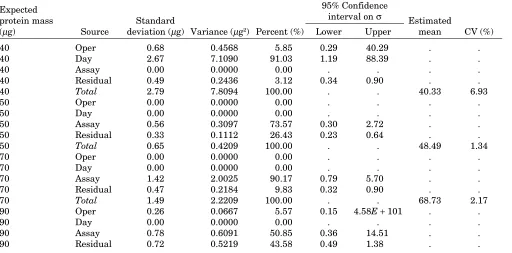
For each mass on the Product W curve, the data will be analyzed by variance components analysis (VCA) to estimate the precision components due to InterOperator, InterDay, InterAssay, and Repeatability. For each expected mass, the precision components will be recorded as a variance, standard deviation, and percent of total precision. Nonzero components will be reported with a two-sided 95% confidence interval for the standard deviation. Within each mass, total variance is defined as the sum of the variance components. Total precision will be expressed as a variance, standard deviation, and coefficient of variation (%CV) also called the percent relative standard deviation or %RSD.

(31)

Often, the acceptance criteria are based on design criteria for the development of the method or development data.]

For each mass in the tested range observed, the total %CV must be less than 10%. [These are hypothetical accep-tance criteria. Note that the precision accepaccep-tance criterion can be on the standard deviation or some other metric of variabil-ity, preferably a metric that is somewhat consistent in value over the range of the assay.]

§6.3. Linearity

Within each of the assays A, B, C, and D, least squares linear regression of observed mass will be regressed on expected mass. The linear regression statistics of intercept, slope, correlation coefficient (r), coefficient of determination (r2_{), sum}

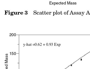
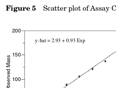
of squares error, and root mean square error will be reported. Lack-of-fit analysis will be performed and reported. For each assay, scatter plots of the data and the least squares regression line will be presented.

For each assay, the coefficient of determination must be greater than 0.975. [These are hypothetical acceptance criteria. Other metrics for linearity could be used for the acceptance criterion. Note that for precise assays, a significant lack-of-fit may not be a meaningful lack-of-fit, due to a slight but consistent curve or other artifact in the data. If lack-of-fit is used for the acceptance criterion, the requirement should be placed on absolute deviation or percent departure from linearity rather than statistical significance. Often the acceptance criteria are based on design criteria for the development of the method or development data.]

§6.4. Range

Range is defined by the interval where the method has demon-strated acceptable accuracy, precision, and linearity.

§6.5. Other Performance Characteristics

(32)

to determine which performance characteristics need to be evaluated in the validation. Depending on the characteristics addres sed, the validation may need more than one design of experiments.]

§7. Validation Matrix

[A matrix of assays is presented to display the study design over the appropriate factors. For this example (Table 1), the factors are Operator, Day, and Assay. For this example, Assay is defined as the interaction between Operator and Day. Note that this matrix shows a hierarchical, or nested, model as Assay (sample preparation) is uniquely defined by Operator and Day.]

§8. Attachments and Forms

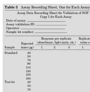
[This section contains forms for documenting that all training requirements have been met, sample preparation instructions as necessary to the execution of the validation experiments, and data recording forms. Places for signatures for perfor-mance and review should be included on each form as appro-priate to company quality and documentation standards. For examples, see Tables 2 and 3.]

Table 1 Matrix of Validation Assays

Assay Day Operator Replicates

A 1 I 3

B 1 II 3

C 2 I 3

D 2 II 3

Four assays with three replicates each. Day 1 is a separate day than Day 2. Table 2 Training Verification to Include Training on Standard Operating Procedure (SOP) 123 and Training on This Validation

Name Department List SOP

Training record complete

Verified by— initials/date

(33)

TERMS AND DEFINITIONS

The following gives definitions of method validation charac-teristics following the references (2,4) ICH Q2A “Text on Validation of Analytical Procedures” and ICH Q2B “Validation of Analytical Procedures: Methodology.” ICH Q2A identifies the validation characteristics that should be evaluated for a variety of analytical methods. ICH Q2B presents guide-lines for carrying out the validation of these characteristics.

Table 3 Assay Recording Sheet, One for Each Assay

Assay Data Recording Sheet for Validation of SOP 123 Copy 1 for Each Assay

Date of assay: Assay validation ID: Operator:

Sample lot number:

Sample

Expected mass (µg)

Response per replicate (absorbance, light units, etc.)

Replicate calibrated value of mass (µg)

1 2 3 1 2 3

Standard 40 50 70 90 110 130 150 180 Test lot 40 50 70 90 110 130 150 180

(34)

The validation characteristics of accuracy, precision, and linearity were presented in the example protocol of the previ-ous section.

Accuracy

Accuracy is a measure of how close to truth a method is in its measurement of a product parameter. In statistical terms, accuracy measures the bias of the method relative to a stan-dard. As accuracy is a relative measurement, we need a defi-nition of “true” or expected value. Often, there is no “gold standard” or independent measurement of the product para-meter. Then, it may be appropriate to use a historical mea-surement of the same sample or a within-method control for comparison. This must be accounted for in the design of exper-iments to be conducted for the validation and spelled out in the protocol. Accuracy is measured by the observed value of the method relative to an expected value for that observation. Accuracy in percent can be calculated as ratio of observed to expected results or as a bias of the ratio of the difference between observed and expected to the expected result. For example, suppose that a standard one-pound brick of gold is measured on a scale 10 times and the average of these 10 weights is 9.99 lbs. Then calculating accuracy as a ratio, the accuracy of the scale can be estimated at (9.99/10) × 100% = 99.90%. Calculating the accuracy as a bias then [(9.99 – 10)/10]

× 100% = −0.10% is the estimated bias. In the first approach ideal accuracy is 100%, and in the second calculation ideal bias is 0%.

Precision and Ruggedness

(35)

(e.g., gels or columns). Variance components measure the con-tribution of each of these external factors to the variability of the method’s results on the same sample of product. To estimate the variance components, the design of validation experiments must be balanced with respect to these factors.

Precision components are defined at three levels: repro-ducibility, intermediate precision, and repeatability. Repro-ducibility is the variability of the method between laboratories or facilities. However, as a laboratory is not “randomly selected” from a large population of facilities, laboratory is a fixed effect. Consequently, the assessment of reproducibility is a question of comparing the average results between labo-ratories. Additionally, the variation observed within labora-tory should be compared to ensure that laboralabora-tory does not have an effect either on the average result of the method or on the variability of the method. To assess reproducibility, conduct the same set of validation experiments within each laboratory and compare both the accuracy results and the precision results. If the differences are meaningful, analysis of variance (ANOVA) tests can be conducted to determine whether there is a statistically significant laboratory effect on the mean or on the variance of the method. For simplicity, the validation discussed within this chapter will not consider reproducibility and only one laboratory is considered.

(36)

ICH Q2A defines repeatability as the variability of the assay results “under the same operating conditions over a short interval of time. Repeatability is also termed intra-assay precision.” A reportable value of an assay is often the average of a specified number of replicate values, where the replicates are processed using the same sample preparation. Thus, it is not possible to obtain a true repeat of the assay’s reportable value. Repeatability can be modeled as the within-assay vari-ability of the replicates; however, it should be noted that this precision is at the level of the replicate and not at the level of the reportable value. If the reportable value is an average of K replicates the variance of the reportable values will be less than that of the replicates by a factor of 1/K (the standard deviation will be less by a factor of (1/ √ K __ ).

Ruggedness is not mentioned in the ICH guidelines. The USP (5) defines ruggedness as “the degree of reproducibility of test results obtained by the analysis of the same samples under a variety of normal test conditions.” Thus, ruggedness also addresses the typical external changes in the execution of the method such as change in day, operator, or assay prepara-tions. Ruggedness and intermediate precision are two sides of the same coin, but they measure different concepts. Inter-mediate precision is measured with a standard deviation or %RSD. Ruggedness is the lack of a factor effect. “Changing the instrument has no effect on the results” is a statement address-ing ruggedness. Ruggedness is modeled as a fixed effect mea-suring the change in average results due to a change in instrument.

Linearity

(37)

experiments are balanced both with respect to the variance components and also over the range of method validation. Thus, the levels of expected input should be evenly spaced across the range of the method with an equal number of obser-vations at each level.

Robustness

Robustness refers to the effect on the assay response due to minor perturbations in sample preparations. In contrast to precision, robustness refers to the minor perturbations of fac-tors internal to the assay (e.g., incubation time, temperature, or amount of reagent) whereas intermediate precision and ruggedness refer to factors necessary in the performance of the method that are external to the assay (day-to-day changes, operator changes, instrument changes). In method develop-ment, acceptable ranges for assay input parameters should be found where the assay response stays fairly constant. In these ranges the method is said to be robust. To quote for Q2B of the ICH Guidelines: “The evaluation of robustness should be con-sidered during the development phase and depends on the type of procedure under study. It should show the reliability of an analysis with respect to deliberate variations in method parameters (2).”

DESIGN OF EXPERIMENTS Terms and Definitions

Factors, Levels, and Treatments

(38)

Fixed Effects, Random Effects, Main Effects, and Interactions

Factors are fixed if the “values” of the levels are given or do not vary. Factors are random if the value is, for pragmatic purposes, randomly selected from a population of all values. To illuminate in an example: if a small lab has two analysts that will always be running the assays then the factor “ana-lyst” is considered fixed with two levels (one level for analyst 1, the other level for analyst 2); however, if the lab is large and/or there is a high turnover in analysts then for each run of an assay the “analyst” could be regarded as selected at random among a population of trained analysts.

In a statistical model, fixed effects have an influence on the mean value or average of the method’s response while random effects have an influence on the variability of the method. Fixed effects are assessed in the context of accuracy. Random effects are assessed in the context of precision and become the inter mediate precision components. In designing the validation design matrix the validation assays need to be balanced over both the fixed effects and the random effects. A mixed effects model (or design) occurs when both fixed effects and random effects are present (6).

Only one lot of well-characterized product or reference standard should be used in the validation. Product lot or batch is not a factor in method validation. Factors that are typically assessed are instrument or machine, analyst or operator, day, and other factors external to the method itself that come into play in the typical running of an assay.

(39)

average response between the low and high levels of factor A when factor B is high then there is an interaction between factor A and factor B. Figure 1 shows an interaction between time and temperature.

Nested and Crossed Factors

Factor A is nested within factor B if the levels of factor A change with the level of factor B. For example, if batches or lots are tested by taking samples from the production line and then aliquots are taken from each sample, then the aliquots are nested within the samples which are nested within the batches (7). Factors C and D are crossed if all levels of factor C can occur with all levels of factor D. For example, in the sample protocol of section IIB, days and operators are crossed, as each of the two operators perform an assay on each of two the days.

Aliasing and Confounding

If each level of one factor only occurs at a specific level of another factor, then the two factors are said to be confounded. When confounding or aliasing occurs, the data analysis cannot distinguish between the effects of the two confounded factors. Figure 1 Interaction between time and temperature. The response profile to time depends on the temperature.

Interaction Between Time and Temperature

0 50 100 150 200 250

2 hours 3 hours 4 hours Time (hours)

Response

(40)

If a significant effect is apparent it is impossible to tell which factor is responsible for the effect. In designing experiments, the number of treatments or experimental trials can be reduced by intentionally aliasing one factor with another. For example, a main effect can be aliased with a high-order inter-action, especially if it is a reasonable assumption that the interaction effect does not exist or is negligible.

Experimental Designs

In this section, three categories of experimental design are considered for method validation experiments. An important quality of the design to be used is balance. Balance occurs when the levels each factor (either a fixed effects factor or a random effects variance component) are assigned the same number of experimental trials. Lack of balance can lead to erroneous statistical estimates of accuracy, precision, and lin-earity. Balance of design is one of the most important consid-erations in setting up the experimental trials. From a heuristic view this makes sense, we want an equivalent amount of information from each level of the factors.

Full Factorial Designs

A full factorial design is one in which every level of each factor occurs for every combination of the levels of the other factors. If each of n factor has two levels, frequently denoted “+” for one level and “–” for the other level, then the number of treatments is two raised to the nth power. Full factorial designs when each factor has the same number of levels are referred to as kn

facto-rial designs, where k is the number of levels and n is the number of factors, as kn_{is the number of treatments needed. If factor}

A has three levels, factor B has two levels, and factor C has three levels then a full factorial design has 3 × 2 × 3 = 18 treat-ments or experimental trials.

(41)

factor B, and factor C, each with three levels, is shown in the design matrix presented in Table 4.

Fractional Factorial Designs

Often a full factorial design requires too many resources and an experimental design with fewer treatments is required. Fractional factorials can reduce the number of experimental trials by aliasing one or more of the factors with other factors or interactions of factors. A fractional factorial of a full facto-rial design 2n_{cuts the number of trials or treatments by1/2,}

1/4, or 1/2p_{. When the number of experimental trials is reduced}

from 2n_{by a factor of 1/2}p_{. the design is referred to as a 2}n–p

fractional factorial. The full factorial design (23_{factorial design} with eight treatments) presented in Table 4 can be reduced to a 23–1_{fractional factorial design with four experimental trials} if factor C is aliased with the two-factor interaction of factors A and B. The resulting design is presented in Table 5. Note that the effect of factor C is confounded with the interaction of factors A and B. This can be observed in the design matrix by multiplying the levels of factors A and B to get the level of factor C (+×+= +, +×−=−, and − × −=+).

The resolution of a design is a categorization of the alias-ing in the design. For resolution III design, main effects are not aliased with each other but each main effect is aliased Table 4 Full Factorial Design for Three Factors, Factors A, B, and C, Each with Two Levels, Low (−) and High (+)

Treatment Factor A Factor B Factor C

1 − − −

2 + − −

3 − + −

4 + + −

5 − − +

6 + − +

7 − + +

8 + + +

(42)

with two-factor interactions. In a resolution IV design, some main effects are aliased with three-factor interactions and two-factor interactions are aliased with each other (2–4). The design shown in Table 5 is resolution III, as main effect of factor C is aliased with the interaction between factors A and B. Also, A is aliased with B and C, and B is aliased with A and C. Resolution of design is discussed in more detail in most texts on experimental design including John (6), Box, Hunter, and Hunter (7), and Kuehl (8).

Plackett-Burman Designs

Plackett-Burman designs are a group of orthogonal array designs of resolution III, where the number of experimental trials is a multiple of four, but is not a power of two. In most Plackett-Burman designs each factor has exactly two levels. These designs are useful as they require fewer resources. Placket-Burman designs are used to estimate main effects only. The reader is referred to the references (6–8) on experi-mental design for listings of Plackett-Burman designs.

Designs for Quantitative Method Validation

Full factorial designs can be used in quantitative method val-idation. With very few factors this is a feasible design. A simple way to display the experiment necessary for the vali-dation is to display the assay runs in a table or matrix. For instance, suppose a method is run on two different machines and the goal is to assess intermediate precision components. We have the random effects of operator and day and a fixed Table 5 Fractional Factorial Design for Three Factors, Factors A, B, and C, Each with Two Levels, Low (−) and High (+)

Treatment Factor A Factor B Factor C

1 − − +

2 + + +

3 − + −

4 + − −

(43)

effect due to machine. If the factors operator and day each have two levels, the full factorial design is shown in Table 4 with factor A as operator, factor B as day, and factor C as machine. Eight assays will be run; the replicates of the assays will be used in estimating repeatability. All factors are crossed with each other.

The full factorial design may not be practical. Perhaps it is not possible for one operator to run two assays on one day. Then a fractional factorial design can be used. The design shown in Table 5 is resolution III design with four experimen-tal trials. As machine is aliased with the interaction between operator and day, the main effect due to machine can be esti-mated only if we assume there is negligible interaction between operator and day. Often, interactions can be assumed to be negligible based on prior knowledge or the science that is known about the situation.

The design shown in Table 5 is also the design of the example protocol. In the example protocol the third factor is assay. The effect of assay is aliased with the interaction of operator and day, and assay is also nested within the interac-tion. Note that if the design of Table 4 were used, and two assays were run for each operator and day combination, then assay would still be nested within the interaction. Each time an assay is run, it is a different assay; hence, the number of levels of the factor assay is just the number of assays that are run. However, running two assays within each operator and day combination will give a better empirical estimate of inter-assay variability but inter-assay effect cannot be estimated inde-pendently of the interaction. This is because assay takes on a different “value” each time the assay is run. (In contrast, in the previous example the third-factor machine is crossed with the factors operator and day; consequently, the machine effect can be estimated independently of operator and day effects.)

(44)

least five levels evenly spaced across the range to be validated. For example in validating a method that measures concentra-tion of an analyte, the sample being tested would be diluted out to (or concentrated to) five expected concentrations evenly spaced between 20% below the lower limit of the method’s stated range and 20% above the upper limit of the method’s stated range. In an assay that can measure multiple concen-trations simultaneously, each assay would test these five diluted samples in K-replicates (within-assay replicates; the assay’s reportable value could be the average of these K repli-cates). If this procedure is repeated using I operators over J days then the method characteristics of accuracy, precision, and linearity can be assessed with one set of I× J assays. In essence, the factor concentration is crossed with the other fac-tors as each of the five concentrations is run in all of the assays. In the example protocol, eight levels of mass are used.

STATISTICAL ANALYSES

The experimental design selected, as well as the type of fac-tors in the design, dictates the statistical model to be used for data analysis. As mentioned previously, fixed effects influence the mean value of a response, while random effects influence the variance. In this validation, the model has at least one fixed effect of the overall average response and the intermedi-ate precision components are random effects. When a statisti-cal model has both fixed effects and random effects it is statisti-called a mixed effects model.

The statistical software package SAS®_{(SAS Institute} Inc., Cary, North Carolina, U.S.A.) has a module [PROC MIXED (10)], which analyzes mixed effects models and pro-vides estimates for both the fixed (shifts on the mean) and random effects (variance components estimates).

(45)

divided by expected mass as a percentage. For precision the response variable is observed mass. Both the accuracy and the precision results are reported for each expected mass. The lin-earity assessment uses the entire data set over all expected masses. Consequently, the root mean square error (RMSE) from the linearity analysis can be viewed as measurement of overall repeatability.

ANOVA can be used to test whether the fixed effects are significant. For example, if there is a factor machine with two levels (representing two machines), an ANOVA can be used to estimate machine effect. If the difference between the average responses for each machine is not meaningfully different, and the variance components within each machine are similar, then the variance components can be analyzed averaging over the machines. If there is a meaningful difference between the two observed machine averages, then an F-test can be used to test whether machine effect is significant.

Accuracy is estimated from the fixed effects components of the model. If the overall mean is the only fixed effect, then accuracy is reported as the estimate of the overall mean accu-racy with a 95% confidence interval. As the standard error will be calculated from a variance components estimate includ-ing intermediate precision components and repeatability, the degrees of freedom can be calculated using Satterthwaite’s approximation (6). The software program SAS has a proce-dure for mixed model analysis (PROC MIXED); PROC MIXED has an option to use Satterthwaite’s degrees of freedom in cal-culating the confidence interval for the mean accuracy. An example program and output is shown later for the example protocol.

(46)

many textbooks, including Searle et al. (11) which provides an in-depth discussion of variance components estimation. Ano-ther method is to use maximum likelihood estimation (MLE). Both of these approaches have drawbacks. ANOVA estimates can be negative as they are a linear combination of sums of squares and there is nothing inherent in restricting the result-ing estimates to be nonnegative. Maximum likelihood esti-mates can be biased as the estimators do not factor in the number of fixed effects being estimated in the model. A third approach is to use maximum likelihood and restrict the domain of the variance estimates to nonnegative values by “estimat-ing variance components based on residuals calculated after fitting by ordinary least squares just the fixed effects part of the model” (11); this is known as restricted maximum likeli-hood estimation (REML). If the design is balanced (i.e., there are the same number of assays run per each day, per each operator, and so on) and the ANOVA estimates are nonnega-tive, then theoretically the REML estimates and the ANOVA estimates agree. SAS’s PROC MIXED has options for all of these methods of estimation. The example protocol analysis shows use of REML. For any of these methods, it is very impor-tant that the original design of experiments is balanced to get statistically sound estimates of variance components.

The basic idea behind variance components estimation is that the variability of the data is parsed out to the random effects of the model. For example, operator-to-operator vari-ability can be assessed roughly by calculating the standard deviation of the operator-specific averages. Thus, it is clear why balance is very important; if the data are not balanced then we are comparing averages from differing number of values, thus the average with the smaller sample size is more variable than that with the larger sample size (i.e., we are mixing apples with oranges).

(47)

Linearity is analyzed using least squares regression of the observed responses against the expected responses, or the regression of the observed responses against the amount of analyte in the sample. The linearity here is of the reportable value versus the amount of analyte in the sample. Note, in the example protocol the responses are the replicate values for each assay at each mass; the average of three within-assay replicates is the reportable value (at each mass) of SOP 123 (in release testing, only one reportable value, the average of three replicates, is reported as the mass of the sample is unknown). If the entire range is assayed in each assay (as in the example validation), then linearity can be assessed within each assay or over all assays. If linearity is assessed using all the data then the RMSE can be used as a measure of overall precision as all the assays over all days and operators are rep-resented. If linearity is assessed within each assay then the RMSE is another measure of repeatability (measurement of error variability within assay).

When there is more than one observation (whether it be replicate values or more than one reportable value over a number of assays) at each level of the analyte, then a lack-of-fit analysis can be conducted. This analysis tests whether the average response at each level of the analyte is a significantly better model for average assay response than the linear model. A significant lack-of-fit can exist even with a high correlation coefficient (or high coefficient of determination) and the maxi-mum deviation of response from the predicted value of the line should be assessed for practical significance.

EXAMPLE VALIDATION DATA ANALYSIS

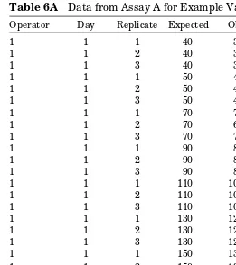
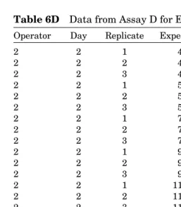
The data are collected and recorded in tables (Tables 6A–D for hypothetical data). The validation characteristics of accuracy, precision, and linearity are analyzed from the data for this example validation.

Model for Accuracy and Precision

(48)

mass of 40 µg, 50 µg, 70 µg, 90 µg, 110 µg, 130 µg, 150 µg, and 180 µg:

Yijk=µ+ Opi+ Dayj+ Assay (Op × Day)ij+εijk (1)

Here, Y is the response variable. For accuracy, Y is observed mass divided by expected mass expressed as a percent, % accuracy (note that this is measuring percent recovery against an expected value). For precision, Y is observed mass. The term µ is a fixed effect representing the population overall average mass for each expected mass. The term Op is the random component added by operator i; Day is the random component added by day j; and Assay is nested in the interac-tion of operator and day. The term ε is the random error of replicate k of the assay performed by operator i on day j. Table 6A Data from Assay A for Example Validation

Operator Day Replicate Expected Observed

1 1 1 40 38.7398

1 1 2 40 38.6092

1 1 3 40 39.0990

1 1 1 50 49.4436

1 1 2 50 48.7904

1 1 3 50 48.6924

1 1 1 70 70.6760

1 1 2 70 69.5980

1 1 3 70 70.2180

1 1 1 90 88.7400

1 1 2 90 87.7280

1 1 3 90 88.4780

1 1 1 110 106.3140

1 1 2 110 105.2700

1 1 3 110 106.3780

1 1 1 130 123.5940

1 1 2 130 122.5820

1 1 3 130 122.1900

1 1 1 150 138.5220

1 1 2 150 138.9480

1 1 3 150 138.9480

1 1 1 180 172.9140

1 1 2 180 172.2600

(49)

Average accuracy is estimated by the overall observed accuracy. The parameter being estimated is µ. The standard error of this estimate is a function of the variance components for operator, day, assay, and repeatability.

SAS PROC MIXED is used to analyze the data. For accu-racy, the SAS code used is:

*SAS code for Accuracy;

PROC MIXED DATA = example CL; CLASS oper day assay;

MODEL acc = / solution cl ddfm = satterth; RANDOM oper day assay;

BY exp; RUN

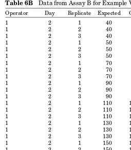
Table 6B Data from Assay B for Example Validation

1 2 1 40 38.0584

1 2 2 40 38.1000

1 2 3 40 38.0450

1 2 1 50 47.6778

1 2 2 50 47.7412

1 2 3 50 48.1222

1 2 1 70 67.4260

1 2 2 70 66.9500

1 2 3 70 66.9500

1 2 1 90 86.7940

1 2 2 90 85.6180

1 2 3 90 86.1580

1 2 1 110 103.4300

1 2 2 110 101.6200

1 2 3 110 102.0960

1 2 1 130 118.4780

1 2 2 130 117.4940

1 2 3 130 118.2260

1 2 1 150 134.7020

1 2 2 150 132.1940

1 2 3 150 132.5440

1 2 1 180 179.2500

1 2 2 180 172.1000

(50)

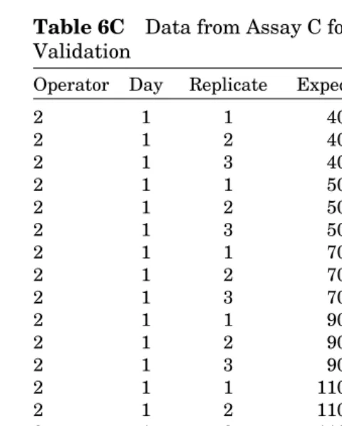
In the code, “oper” reads in the level of operator, “day” reads in the level of day, “assay” reads in the assay, “acc” is Y for accuracy and is defined by the ratio of observed mass to expected mass (“exp”). Note that the “BY exp” the procedure is run separately for each level of the expected mass using “exp” as the variable name. In this manner, the precision of the accuracy and the variance components are estimated inde-pendently at each level of the expected mass. Thus, we obtain “picture” of the assay’s performance characteristics across the operational range. As assay is nested in the interaction between operator and day, the same analysis can be coded used “oper* day” in place of “assay” in the previuos code. The “CL” and “cl” in the procedure line and model statement are Table 6C Data from Assay C for Example

Validation

2 1 1 40 41.7500

2 1 2 40 43.2800

2 1 3 40 43.5100

2 1 1 50 48.1538

2 1 2 50 47.9650

2 1 3 50 48.3110

2 1 1 70 67.9920

2 1 2 70 67.8340

2 1 3 70 68.0220

2 1 1 90 88.6140

2 1 2 90 87.1980

2 1 3 90 86.9780

2 1 1 110 104.1140

2 1 2 110 103.3580

2 1 3 110 103.6100

2 1 1 130 119.9580

2 1 2 130 119.4560

2 1 3 130 119.2360

2 1 1 150 136.9660

2 1 2 150 133.6340

2 1 3 150 134.3260

2 1 1 180 179.1500

2 1 2 180 178.2500

(51)

calls for confidence limits. In the model statement “ddfm = satterth” calls for Satterthwaite’s degrees of freedom (see Ref. 6 for a discussion of Satterthwaite’s approximation) to be used in calculating the confidence limits.

Model (1) is used for precision analysis. For precision, Y is the observed mass (rather than observed mass divided by expected mass). Each random effects component (operator, day, assay, and error or repeatability) contributes to the total variance of Y. The total variance of Y is defined as the sum of

variance components for operator, day, assay, and repeatabil-ity, respectively, then total variance is σ 2

Table 6D Data from Assay D for Example Validation

(52)

For precision, the SAS code used is shown next. Note that the only change is the Y value; for precision, Y is observed mass, called “obt” in the code.

*SAS code for Precision;

PROC MIXED DATA = example CL; CLASS oper day assay;

MODEL obt = / solution cl ddfm = satterth; RANDOM oper day assay;

BY exp; RUN

This program will give variance estimates for each of the pre-cision components along with two-sided 95% confidence inter-vals for the population variance component for each expected mass. SAS PROC MIXED will provide ANOVA estimates, maximum likelihood estimates, and REML estimates; the default estimation, used here, is REML.

Method of moments estimates (also known as ANOVA estimates) can be calculated directly from the raw data as long as the design is balanced. The reader is referred to Searle et al. (11) for a thorough but rather technical presentation of variance components analysis. The equations that follow show the ANOVA estimates for the validation example. First, a two-factor with interaction ANOVA table is computed (Table 7). Then the observed mean squares are equated to the expected mean squares and solved for the variance compo-nents (Table 8 and the equations that follow).

The expected mean squares are equated to the observed mean squares (those from the data) and solved for the vari-ance components. Thus, σˆ 2

ε = MSE is the variance estimate

for repeatability, σˆ 2 Assay =

MSA – MSE

_________ _m is the variance estimate for assay, σˆ 2

Day = __________ MSD – MSAa·m is the variance estimate for day,

and σˆ 2

(53)

Linearity Analysis

For the example validation, linearity will be analyzed within each assay and across all four assays. For the second analysis, as mentioned before, the RMSE can be used as a measure of Table 7 Analysis of Variance (ANOVA), Sum of Squares and Mean Square Formulae for a Two-Factor Mixed Model with Interaction for the Validation Matrix of Tables 4 or 5 to be Used in ANOVA

Variance Component Estimation

Source df Sum of squares

Mean

Here, a bar over the Y indicates averaging over the missing subscript(s); the subscript “i” is an index for operator, the subscript “j” is an index for day, assay is indexed by must be balanced for these formulas to apply.

Abbreviations: a, number of operators; b, number of days; m, number of replicates; df,

degrees of freedom.

Source: From Ref. 11.

Table 8 Expected Mean Squares for the Two-Factor with Interaction Analysis of Variance Table Shown in Table 7

Source Mean square Expected mean square