A FEASIBILITY STUDY ON USING ViSP’S 3D MODEL-BASED TRACKER FOR
UAV POSE ESTIMATION IN OUTDOOR ENVIRONMENTS
Julien Li-Chee-Ming and Costas Armenakis
Geomatics Engineering, GeoICT Lab
Department of Earth and Space Science and Engineering Lassonde School of Engineering, York University
4700 Keele Str., Toronto, Ontario, M3J 1P3 {julienli}, {armenc} @yorku.ca
Commission I, ICWG I/Vb
KEYWORDS: UAV, Close Range Photogrammetry, Mapping, Tracking, Robotics, Navigation, Object Recognition, Augmented Reality, ViSP
ABSTRACT:
This paper presents a novel application of the Visual Servoing Platform’s (ViSP) for small UAV pose estimation in outdoor environments. Given an initial approximation for the camera position and orientation, or camera pose, ViSP automatically establishes and continuously tracks corresponding features between an image sequence and a 3D wireframe model of the environment. As ViSP has been demonstrated to perform well in small and cluttered indoor environments, this paper explores the application of ViSP for UAV mapping of outdoor landscapes and tracking of large objects (i.e. building models). Our presented experiments demonstrate the data obtainable by the UAV, assess ViSP’s data processing strategies, and evaluate the performance of the tracker.
1. INTRODUCTION
Precise navigation is required for UAVs operating in GPS denied environments, or in dense-multipath environments such as urban canyons. This is especially useful in urban missions, where the possibility of crashing is high, as UAVs fly at low altitudes among buildings and in strong winds, whiles avoiding obstacles and performing sharp maneuvers. The GeoICT Lab at York University is developing mapping and tracking systems based on small unmanned aerial systems such as the Aeryon Scout quadrotor small UAV (Unmanned Aerial Vehicle) (Aeryon, 2015). The Scout is equipped with a single frequency GPS sensor that provides positioning accuracies of about 3 m, and an Attitude and Heading Reference System (AHRS) that estimates attitude to about 3°. It is also equipped with a small forward-looking FPV (First Person Viewing) video camera and a transmitter to downlink the video signal wirelessly in real-time to a monitoring ground station or to virtual reality goggles. FPV gives the operator of a radio-controlled UAV a perspective view from the ‘cockpit’. This augments the visual line-of-sight, offering additional situation awareness. FPV systems are used solely as a visual aid in remotely piloting the aircraft.
We have proposed a method to further extend the application of this system by estimating the pose (i.e. position and orientation) of the UAV from the FPV video as it travels through a known 3D environment. We have applied a geometric hashing based method to match the extracted linear features from the FPV video images with a database of vertical line features extracted from synthetic images of the 3D building models (Li-Chee Ming and Armenakis, 2014). Sub-meter positional accuracies in the object space were achieved when proper viewing geometric configuration, control points, and tie points are used. The obtained quantitative information on position and orientation of the aerial platform supports the UAV operator in navigation and path planning. If an autopilot is available, this system may also be used to improve the navigation solution’s position and orientation.
2. VISUAL SERVOING AND VISUAL TRACKING
In this paper we extend on our previous work where a 3D CAD model of the environment is available. We assess the Visual Servoing Platform’s (ViSP) registration techniques which provide continuous tracking and alignment of features extracted from the FPV video image (in real-time) and the 3D model of the environment (Marchand and Chaumette, 2005). ViSP provides tracking techniques that are divided into two classes: feature-based and model-based tracking. The first approach focuses on tracking 2D geometric primitives in the image, such as points (Shi and Tomasi, 1994), straight line segments (Smith et al., 2006), circles or ellipses (Vincze, 2001), or object contours (Blake and Isard, 1998). However, ViSP does not provide a means to match these tracked image features with the 3D model, which is required in the georeferencing process. The second method is more suitable because it explicitly uses a 3D model of the object in the tracking algorithm. Further, a by-product of this tracking method is the 3D camera pose, which is our main objective. This second class of methods usually provides a more robust solution (for example, it handles partial occlusion of the objects, and shadows).
2.1 The Moving Edges Tracker
The moving edges algorithm (Boutemy, 1989) matches image edges in the video image frames to the 3D model’s edges, which are called model contours in ViSP. The required initial approximation of the camera pose is provided by the UAV’s autopilot GPS positioning, and orientation from the AHRS. Observations from these sensors are no longer used after initializing the camera pose in order to assess ViSP’s tracking performance.
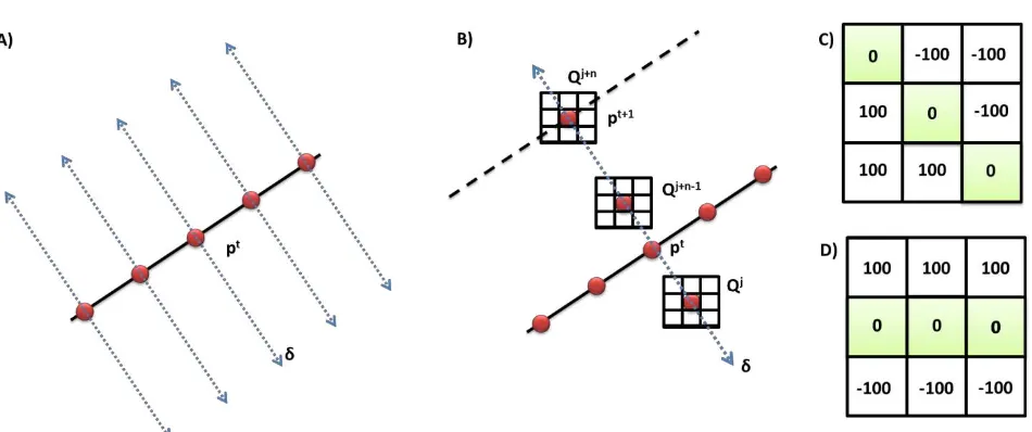
The process consists of searching for the corresponding point pt+1 in the image It+1 for each point pt. A 1D search interval {Qj, j [-J, J] } is determined in the direction δ of the normal to the contour. For each position Qj lying the direction δ, a mask convolution Mδ corresponding to the square root of a log-likelihood ratio ζj is computed as a similarity measure. Thus the new position pt+1 is given by:
�
�∗= argmax
�∈[−�,�]
�
�(1)
with
��
= |�
�(��)�+1∗ ��
+ �
�(� �)∗ ��|
(2)
υ(.) is the neighbourhood of the considered pixel, ViSP’s default is a 7x7 pixel mask (Comport et al., 2003).
Figure 1. ViSP’s pose estimation workflow.
Figure 2. Determining point position in the next image using the oriented gradient algorithm: A) calculating the normal at sample points, B) Sampling along the normal, C)-D) 2 out of the 180 3x3 predetermined masks, C) 180o, D) 45o (Comport et al., 2003).
Model contours are sampled at a user specified distance interval (Figure 2A). At these sample points (e.g. pt), a one dimensional search is performed along the normal direction (δ) of the contour for corresponding image edges (Figure 2B). An oriented gradient mask is used to detect edges (e.g. Figures 2C and 2D). One of the advantages of this method is that it only searches for image edges which are oriented in the same direction as the model contour. An array of 180 masks is generated off-line which is indexed according to the contour angle. The run-time is limited only by the efficiency of the convolution, which leads to real-time performance (Comport et al., 2003). Line segments are favourable features to track because the choice of the convolution mask is simply made using the slope of the contour line. There are trade-offs to be made between real-time performance and both mask size and search distance.
2.2 Virtual Visual Servoing
∆=
� −
�= [�
��, � −
�](3)
where � � �, � is the projection model according to the intrinsic parameters ξ and camera pose r, expressed in the object frame. It is assumed the intrinsic parameters are available, but VVS can estimate them along with the extrinsic parameters. An iteratively re-weighted least squares (IRLS) implementation of the M-estimator is used to minimize the error of the summation ∆ squares. IRLS was chosen over other M-estimators because it is capable of statistically rejecting outliers.
Comport et al. (2003) provide the derivation of ViSP’s control law. If the corresponding features are well chosen, there is only one camera pose that allows the minimization to be achieved. Conversely, convergence may not be obtained if the error is too large.
2.3 TIN to Polygon 3D Model
ViSP specifies that a 3D model of the object to track should be represented using VRML (Virtual Reality Modeling Language). The model needs to respect two conditions:
1) The faces of the modelled object have to be oriented so that their normal goes out of the object. The tracker uses the normal to determine if a face is visible.
2) The faces of the model are not systematically modelled by triangles. The lines that appear in the model must match image edges.
Due to the second condition, the 3D building models used in the experiments had to be converted from TIN (Triangulated Irregular Network) to 3D polygon models. The algorithm developed to solve this problem is as follows:
1) Region growing that groups connected triangles with parallel normals.
2) Extract the outline of each group to use as the new polygon faces.
The region growing algorithm was implemented as a recursive function. A seed triangle (selected arbitrarily from the TIN model) searches for its neighbouring triangles, that is, triangles that share a side with it, and have parallel normals. The neighbouring triangles are added to the seed’s group. Then each neighbour looks for its own neighbours. The function terminates if all the neighbours have been visited or a side does not have a neighbour. For example, the blue triangles in Figure 3 belong to one group.
Once all of the triangles have been grouped, the outline of each group is determined (the black line in Figure 3). Firstly, all of edges that belong to only one triangle are identified, these are the outlining edges. These unshared edges are then ordered so the end of one edge connects to the start of another. The first edge is chosen arbitrarily.
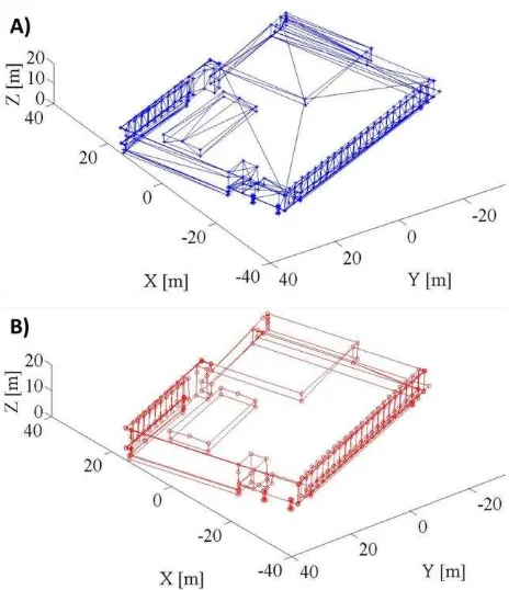
Figure 4A shows the 3D TIN model of York University’s Lassonde Buillding. Figure 4B shows the resulting polygon model of the same building.
3. RESULTS AND DISCUSSION
The 3D virtual building model of York University’s Keele Campus campus (Armenakis and Sohn, 2009) was used as a known environment. The model consists of photorealistic 3D TIN reconstructions of buildings, trees, and terrain (Figure 5).
reconstructions of buildings, trees, and terrain. The model was generated from building footprint vector data, Digital Surface Model (DSM) with 0.75m ground spacing, corresponding orthophotos at 0.15 m spatial resolution and terrestrial images. The 3D building models were further refined with airborne lidar data having a point density of 1.9 points per square metre (Corral-Soto et al., 2012).
Figure 3. An example of region growing and outline detection: The blue triangles belong to a group because one triangle is connected to at least one other triangle with a parallel normal. The outline of the group (black line) consists of the edges that belong only to one triangle.
The 3D CAD model serves two purposes in the proposed approach. Firstly, it provides the necessary level of detail such that individual buildings can be uniquely identified via ViSP’s moving edges algorithm. Secondly, it provides ground control points to photogrammetrically estimate the camera pose. The geometric accuracy of the building models is in the order of 10 to 40 cm.
In our tests we used the data of an Aeryon Scout quadcopter which flew over York University, up to approximately 40 metres above the ground, while its onboard camera focused on buildings, walkways, and trees. Figure 6 shows the UAV’s flight path for the presented experiment.
Figure 5. York University's 3D campus model
Figure 6. Aeryon Scout’s flight path over the Lassonde building
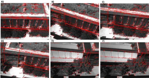
Figure 8. Additional sample frames demonstrating ViSP’s model-based tracker. The East side of York University’s Lassonde Building is being observed, the 3D building model is projected onto the image plane (red lines) using the respective camera intrinsic and extrinsic parameters. Harris corners (red crosses with IDs) are also being tracked.
The camera’s intrinsic parameters were calibrated beforehand and held fixed in the pose estimation process. The image frames were tested at 480p, 720p, and 1080p resolutions. The trials revealed that, at 40 metres above ground level, 480p video performed the best in terms of processing speed and tracking performance. The tracking performance improved because the noisy edges detected by the Moving Edges Tracker at higher resolutions were removed at lower resolutions, leaving only the stronger edge responses.
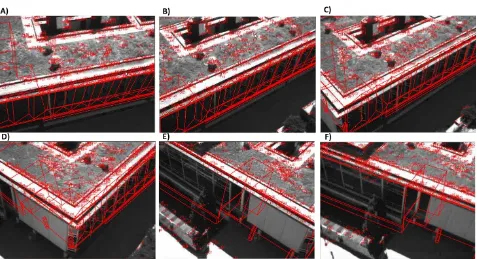
1137 frames were processed at 6 frames per second. Figure 7A-F shows several results from the tracking along the West side and North side of the Lassonde Building. The red lines are the projections of the 3D building model onto the image plane using the respective camera pose. It is evident that, although the tracker does not diverge, there is misalignment between the image and the projected model; this is due to error in the camera pose. Figure 8A-F shows results from ViSP along the East side of the Lassonde Building. Notably, from frame E) to F) in both Figure 7 and 8, ViSP’s robust control law decreases the misalignment between the image and model.
Figure 9 shows a comparison between the UAV’s trajectory according to the onboard GPS versus ViSP’s solution. Figure 10A-C shows the positional coordinates in the X, Y, and Z axes, respectively, from the GPS solution and ViSP’s solution. Figure 10D shows the coordinate differences between the two solutions, and Table 1 provides the average coordinate differences, along with the standard deviations. These figures show gaps in ViSP’s trajectory from when tracking was lost. This was the result from a lack of model features in the camera’s field of view, and because of rapid motions due to the unstabilized camera.
The camera was attached the UAV using a pan-tilt mount, so the camera pitched and yawed independently from the UAV. Therefore, the AHRS’ roll and pitch axes did not align with
the camera frame. However, for both the AHRS’ and ViSP’s the direction cosine matrix rotation sequences are ZYX, thus their Z-axes are parallel. The camera did not pan throughout the flight, so there was a constant offset between the AHRS and camera yaw angles (60.125o).
Figure 10. Positional coordinate comparison between the GPS solution and ViSP’s solution.
Table 1. Mean and standard deviation for the difference in the UAV’s positional coordinates from its onboard GPS and ViSP.
Mean Standard
Deviation
∆X [m] 8.78 ±9.23
∆Y [m] -1.19 ±12.16
∆Z [m] 6.65 ±2.73
∆ψ[o
] 0.15 ±13.87
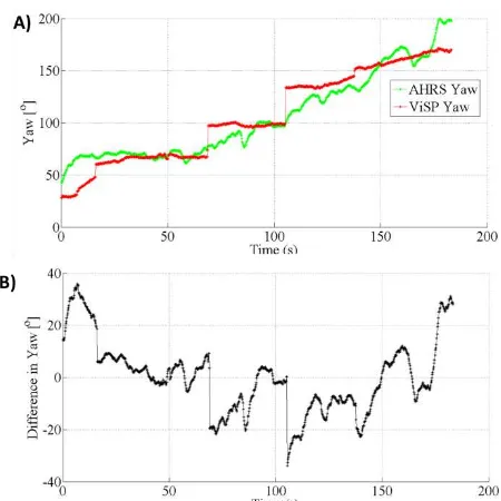
Figure 11A shows the yaw angles, after removing the offset, and Figure 11B shows the difference. It is evident that ViSP’s yaw estimate agrees well with the AHRS solution. The jumps in the data again show where tracking was lost and reset. Table 1 provides the mean difference in yaw (∆ψ), along with its standard deviation.
Figure 11. Yaw angle comparison between the GPS solution and ViSP’s solution.
The experiments suggested that ViSP can provide only an initial approximation for camera pose. This is because the Moving Edges Tracker is a local matching algorithm. A simultaneous bundle adjustment will globally optimize the camera poses, leading to an increase in the accuracies. Figures 7 and 8 show red points that are labelled with their ID numbers, these are Harris corners being tracked using a KLT tracker (Lucas and Kanade, 1981). They may be used as tie points in the bundle adjustment to further optimize the camera poses and generate a sparse point cloud. Dense matching (Rothermel et al., 2012) could be used to increase the point cloud’s density. The Iterative Closest Point (ICP) algorithm (Besl and McKay, 1992) may then be used to refine the alignment between the point cloud and the 3D building model; this should further increase the camera pose accuracies. As both large-scale bundle adjustment, dense matching, and ICP are computationally intensive, they should be done in a post-processing stage.
The real-time camera pose accuracies can be improved by augmenting ViSP’s pose estimate with another pose estimation system. For instance, one could integrate ViSP’s pose with the positional and orientation data from the UAV’s onboard GPS and AHRS, respectively, through a Kalman filter. This would both increase the accuracy of the pose and bridge GPS gaps.
4. CONCLUSIONS AND FUTURE WORK
ACKNOWLEDMENTS
NSERC’s financial support for this research work through a Discovery Grant is much appreciated. We thank Professor James Elder’s Human & Computer Vision Lab in York University’s Centre for Vision Research for providing the UAS video data. Special thanks are given to the members of York University’s GeoICT Lab Damir Gumerov, Yoonseok Jwa, Brian Kim, and Yu Gao, who contributed to the generation of the York University 3D Virtual Campus Model.
REFERENCES
Aeryon. 2015. Aeryon Scout Brochure. Retrieved from www.aeryon.com/products/avs/ aeryon-scout.html. (accessed: 14-May-2015).
Armenakis C, and Sohn G. 2009. iCampus: 3D modeling of York University Campus. In Proc. 2009 Conf. of the American Society for Photogrammetry and Remote Sensing, Baltimore, MA, USA.
Besl PJ, and McKay N.D. 1992. A method for registration of 3-D shapes. IEEE Trans. on Pattern Analysis and Machine Intelligence (Los Alamitos, CA, USA: IEEE Computer Society) 14(2): 239–256.
Blake A, and Isard M. 1998. Active Contours. Springer Verlag.
Bouthemy P. 1989. A maximum likelihood framework for determining moving edges. IEEE Trans, on Pattern Analysis and Machine Intelligence. 11(5): 499-511.
Corral-Soto ER, Tal R, Wang L, Persad R, Chao L, Chan S, Hou B, Sohn G, and Elder JH. 2012. 3D Town: The Automatic Urban Awareness Project. In Proc. 9th Conf. on Computer and Robot Vision, Toronto, pp. 433-440.
Comport A, Marchand,E, and Chaumette F. 2003. Robust and real-time image-based tracking for markerless augmented reality. Technical Report 4847. INRIA.
Li-Chee Ming J, and Armenakis C. 2014. Feasibility study for pose estimation of small UAS in known 3D environment using geometric hashing. Photogrammetric Engineering & Remote Sensing, 80(12): 1117–1128
Lucas B.D., and Kanade T. 1981. An iterative image registration technique with an application to stereo vision. In
Int. Joint Conf. on Artificial Intelligence, IJCAI’81, pp. 674 -679.
Marchand E, and Chaumette F. 2005. Feature tracking for visual servoing purposes. Robotics and Autonomous Systems. 52(1): 53-70.
Rothermel M, Wenzel K, Fritsch D, Haala N. 2012. SURE: Photogrammetric surface reconstruction from imagery.
Proceedings LC3D Workshop, Berlin.
Shi Jand Tomasi C. 1994. Good features to track. IEEE Int. Conf. on Computer Vision and Pattern Recognition. pp. 593-600.
Smith P, Reid I, and Davison, A. 2006. Real-time monocular SLAM with straight lines, Proc of the British Machine Vision Conference.
Sundareswaran V, and Behringer R. 1998. Visual servoing-based augmented reality. In IEEE Workshop on Augmented Reality, San Fransisco.
ViSP. 2013. ViSP: Visual servoing platform – Lagadic research platform. Retrieved from
http://www.irisa.fr/lagadic/visp/visp.html. (accessed: 22-May-2015).
Vincze M. 2001. Robust tracking of ellipses at frame rate.