The 3rd International Conference on Mathematics and Statistics (ICoMS-3) Institut Pertanian Bogor, Indonesia, 5-6 Agustus 2008
ESTIMATION OF OUTSTANDING CLAIMS LIABILITY AND
SENSITIVITY ANALYSIS: PROBABILISTIC TREND FAMILY
(PTF) MODEL
1,3
Arif Herlambang,
2Dumaria R Tampubolon
1Student in Department of Matematics, Institut Teknologi Bandung Jl. Ganesa 10 Bandung 40132
2Lecturer in Department of Matematics, Institut Teknologi Bandung Jl. Ganesa 10 Bandung 40132
3 Lecturer in MIPA Department, Universitas Surabaya Jl. Raya Kali Rungkut Surabaya 60292
e-mail : 1,3[email protected] / [email protected] , 2
[email protected]
Abstract. Outstanding claims liability is the insurance companies’ corporate responsibility towards future debt. There are a number of existing models used to estimate the outstanding claims liability for long tail business. However, some of the assumptions imposed on these models are not met by the claims data under consideration. Furthermore, trends in the development year and payment year periods are not taken into account by these models. The Probabilistic Trend Family (PTF) model is developed to overcome these problems.
In this paper, PTF model is described; and the process of estimating the outstanding claims liability, starting from the preliminary analysis of the claims data to the estimation of the outstanding claims liability is explained. Furthermore, the sensitivity of the obtained estimate of the outstanding claims liability is analyzed using a tool called leverage. Leverage can be used to evaluate the robustness of the model used to estimate the outstanding claims liability.
Keywords : Outstanding claims liability, long tail business, development year period, payment year period , probabilistic trend family, sensitivity, leverage.
1. Introduction
In general insurance, claims are not usually paid as soon as they occur. A number of factors may cause delay between the occurrence and reporting of a claim and delay between the time of reporting and settlement of a claim. In some cases it may take many years until the final payment. Lines of business with this characteristic of claims payment are called long tailed business.
General insurance companies are required to set aside (reserve) enough of their premium income to cover future claim payments from past and current policies.
Based on claims experience in the past, a claim analyst tries to forecast a value for the amount of the liability contingent to events which have yet to happen. In the past, the objective was to obtain a forecast of the central estimate of the distribution of the outstanding claims liability. For many years, actuaries have been applying deterministic forecasting methodologies to estimate the outstanding claims liability. However, in order to quantify the uncertainties on the estimate and to predict the distribution of the outstanding claims liability, the problem needs to be approached stochastically. For the last two decades at least, actuaries and statisticians have been developing statistical forecasting models to estimate the outstanding claims liability as well as measuring its uncertainty.
into account by these models. The common causes of this failure to satisfy assumption motivated the development of the statistical modeling framework. The rich family of statistical models in the framework contains assumptions more in keeping with reality. This statistical modeling framework is based on the analysis of the logarithms of the incremental data. Each model in the framework has four components of interest. The first three components are trends in each of the directions: development period, accident period, and payment/calendar period, while the fourth component is the distribution of the data about the trends. This rich family of models is often named as the Probabilistic Trend Family (PTF).
2. Probabilistic Trend Family (PTF) Model
j
The parameters in the accident year direction determine the level from year to year; often the level shows little change over many years, requiring only a few parameters. The parameters in the development year direction represent the trend from one development year to the next. This trend is often linear (on the log scale) across many of the later development years, often requiring only one parameter to describe the tail of the data. The parameters in the payment year direction describe the trend from payment year to payment year. For further explanation about using PTF models to estimate the outstanding claims liability is given below.
3. Example
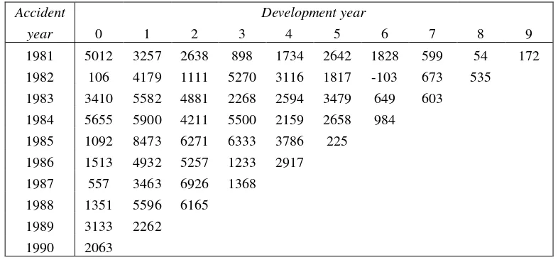
In this paper, we use the data from Mack (1994). The data are incurred losses for automatic facultative business in general liability, taken from the Historical Loss Development Study, 1991, published by the Reinsurance Association of America (data values in thousand dollars).
Table 1 Run-off triangle of the incremental payments of the AFG data
There are some step to estimate the outstanding claims liability using PTF model : 1. Preliminary analysis of the claims data
2. Identification models
3. Estimation outstanding claims liability
solution to solve negative values in the incremental data. Based on Verral and Li method, table 1 can be written
Table 2 Run-off triangle of the incremental payments of the AFG data after modification by constant
solution (
τ
=
Identification models has main goal to built or designed the PTF model that captures trend in the incremental data. After some process (include testing model parameter) there is only one PTF model that can be the optimal model, as we can see in equation (2)
with the values of the parameter
0.1291
The last step is how to calculate the estimation of the outstanding claims liability. From Modification by constant solution
)
τ
−
α
+
γ
+
−
γ
+
σ
=
ˆ
ˆ
2
1
ˆ
)
1
(
ˆ
ˆ
exp
)
,
|
(
p
,i
j
1j
2 2E
i j (4)with parameter values
0.1291
-0.1773
ˆ
0.6054
ˆ
8.1849
ˆ
2 2 1
=
σ
=
γ
=
γ
=
α
.
=
τ
∧
1575.6559
Using equation (4) we get the estimate of the outstanding claims liability
Table 3 the estimate of the outstanding claims liability
Accident Development year
year 0 1 2 3 4 5 6 7 8 9
1981
1982 121.1
1983 450.3 121.1
1984 843.3 450.3 121.1
1985 1312.5 843.3 450.3 121.1
1986 1872.8 1312.5 843.3 450.3 121.1
1987 2541.7 1872.8 1312.5 843.3 450.3 121.1
1988 3340.4 2541.7 1872.8 1312.5 843.3 450.3 121.1
1989 4294.1 3340.4 2541.7 1872.8 1312.5 843.3 450.3 121.1
1990 5432.7 4294.1 3340.4 2541.7 1872.8 1312.5 843.3 450.3 121.1
By adding all cell values at table 3, we get the total estimate of the outstanding claims liability $ 62,042,896 or $ 62 million.
4.
Sensitivity Analysis
In this section we explore the sensitivity of the estimate of the outstanding claims liability, given a particular forecasting method or model. The sensitivity of the estimate will give insights into the method or model chosen and may assist in setting the reserve. Given a forecasting model, the estimate of the outstanding claims liability is dependent on the observed values. Whatever model is used to estimate the outstanding claims liability, it is important to address how sensitive the estimate is to changes in the observed data.
The sensitivity of the obtained estimate of the outstanding claims liability is analyzed using a tool called
leverage. Leverage can be used to evaluate the robustness of the model used to estimate the outstanding claims liability (Tampubolon, 2008).
triangle
off
run
the
of
cell
a
in
payment
l
incrementa
claims
ding
outs
the
of
estimate
Leverage
∆
∆
≡
tan
(5)the value of each cell of a runoff triangle. Sensitivity is measured by making small perturbations in the data because calculating the first partial derivative algebraically is not a simple matter for PTF model. From the definition of a rate of change, a leverage value can be zero, positive or negative. A leverage near zero means that a small perturbation in that particular cell causes (almost) no change in the estimate of the outstanding claims liability. In claims reserving, a forecasting methodology which produces almost zero leverage is not desirable since it means that the estimate is largely independent of the corresponding observed data. A positive leverage, say +k, means that the estimate of the outstanding claims liability is
increased by k times the change in the observed value, whereas a negative leverage of -k, say, means that there is a decrease in the estimate of the outstanding claims liability by the amount of k times the change in the observed value.
3. Empirical Result
To illustrate the procedures, the AFG data described in Section 3 is used. As mentioned earlier, using the PTF model, the estimates of the outstanding claims liability for the AFG data is $ 62.042 million,respectively. Given the PTF model, the PTF leverage is calculated as follows. Let us say that there is a $1000 increase in cell (0,0) of the runoff triangle of the incremental payments (an increase of $1000 is small enough since increases of $500 and $1 in the incremental payments also result in the same leverage values). The resulting leverage is 0.236. This means that there is an increase in the estimate of the outstanding claims liability of almost 0.2 times the increase in the first cell. In other words, had the claims paid in accident year 0 and development year 0 been $5 013 000 instead of $5 012 000, then the resulting PTF estimate of the outstanding claims liability will be approximately $236 higher than the original estimate of $ 62.042 million. In another example, for the same accident year 0, let us say that there is an increase of $1000 in the paid claims at the final development year (at the tail). Then the change in estimated total outstanding is approximately 5 times as much. This means that, had the $1000 claims been paid later, the resulting PTF estimate of the outstanding claims liability will be approximately $5000 higher than the original PTF estimate. So, for the same accident year 0, if the PTF model is used to forecast future values, a lower estimate of the outstanding claims liability will be obtained if the claims were paid earlier and a higher estimate is obtained if they were paid later. The complete leverage values for all of the cells of the runoff triangle of the AFG data are shown in the runoff triangle of the PTF leverage given by table 4. Each cell of the runoff triangle below shows the leverage (the rate of change) of the estimate of the outstanding claims liability at that particular cell.
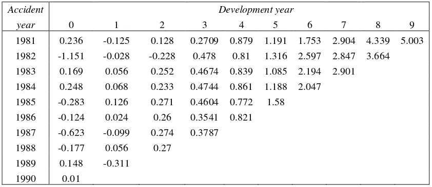
Tabel 4.1 PTF leverage
Accident Development year
year 0 1 2 3 4 5 6 7 8 9 1981 0.236 -0.125 0.128 0.2709 0.879 1.191 1.753 2.904 4.339 5.003 1982 -1.151 -0.028 -0.228 0.478 0.81 1.316 2.597 2.847 3.664 1983 0.169 0.056 0.252 0.4674 0.839 1.085 2.194 2.901
1984 0.248 0.068 0.233 0.4744 0.861 1.188 2.047
1985 -0.283 0.126 0.271 0.4604 0.772 1.58
1986 -0.124 0.024 0.26 0.3541 0.821
1987 -0.623 -0.099 0.274 0.3787
1988 -0.177 0.056 0.27
1989 0.148 -0.311
1990 0.01
Examining table 4, several interesting results may be noted:
2. The PTF leverage values are positive and reasonably high in the tails and for the data in the last accident year, compared to those at the other cells of the runoff triangle. A higher leverage value means that the estimate of the outstanding claims liability is more sensitive to perturbations.
3. For accident year 0 to 6, going across development years, there is a zone of (or close to) zero leverage, at which the PTF method is insensitive to change in the data.
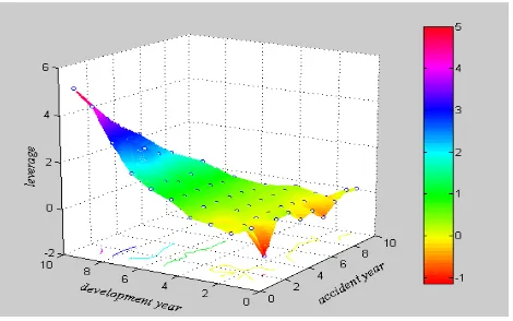
A graphical display of the PTF leverage values of the AFG data is shown in Figure 1. The yellow colour represents zero leverage.
Figure 1. Graphical display of the PTF leverage
References
1. Barnett, G., and Zehnwirth, B. (2000), "Best Estimates for Reserves," Proceedings of the Casualty Actuarial Society, 87, 245-321.
2. Mack, Thomas, “Distribution-Free Calculation of the Standard Error of Chain Ladder Reserve
Estimates,” ASTIN Bulletin, 23, 2, 1993, pp. 213–225.
3. Mack, Thomas, “Which StochasticModel is Underlying the Chain Ladder Method?” Insurance Mathematics and Economics, 15, 2/3, 1994, pp. 133–138.
4. Reinsurance Association of America, Historical Loss Development Study, 1991 Edition, Washington, D.C.: R.A.A., 1991.
5. Tampubolon ,Dumaria R, (2008) ” Uncertainties in the Estimation of Outstanding Claims
Liability in General Insurance”, Ph.D Thesis Macquarie University, Sidney Australia.