Full Terms & Conditions of access and use can be found at
http://www.tandfonline.com/action/journalInformation?journalCode=cbie20
Download by: [Universitas Maritim Raja Ali Haji] Date: 18 January 2016, At: 19:28
ISSN: 0007-4918 (Print) 1472-7234 (Online) Journal homepage: http://www.tandfonline.com/loi/cbie20
Vulnerability of households to health shocks: an
Indonesian study
Nguyen Thi Nhu Nguyet & Eiji Mangyo
To cite this article: Nguyen Thi Nhu Nguyet & Eiji Mangyo (2010) Vulnerability of households to health shocks: an Indonesian study, Bulletin of Indonesian Economic Studies, 46:2, 213-235, DOI: 10.1080/00074918.2010.486108
To link to this article: http://dx.doi.org/10.1080/00074918.2010.486108
Published online: 27 Jul 2010.
Submit your article to this journal
Article views: 144
View related articles
ISSN 0007-4918 print/ISSN 1472-7234 online/10/020213-23 © 2010 Indonesia Project ANU DOI: 10.1080/00074918.2010.486108
VULNERABILITY OF HOUSEHOLDS TO HEALTH SHOCKS:
AN INDONESIAN STUDY
Nguyen Thi Nhu Nguyet* Eiji Mangyo*
United Nations in Viet Nam, Hanoi International University of Japan, Uonuma
We examine the effect of illness and injury shocks on work hours and household consumption in Indonesia. Using indices of activities of daily living to measure health shocks, we ind that both labour hours and household consumption are in-luenced by health shocks to household heads. Further, farm households seem to be more seriously affected than non-farm households by health shocks. However, the magnitude of the health effect on household consumption is small, implying that even farm households are well protected on average by the presence of formal and informal risk-coping mechanisms.
INTRODUCTION
Households can slip into poverty for various reasons, such as macroeconomic and climatic shocks and natural disasters. However, health shocks are generally con-sidered one of the most important triggers of poverty (Dercon 2003; Hoogeveen et al. 2004). Previous empirical studies have used household survey data to exam-ine the impact of health shocks on household welfare in developing countries (Dercon, Hoddinott and Woldehanna 2005; Lindelow and Wagstaff 2005; Yagura 2005; Christiaensen, Hoffmann and Sarris 2007). The vast majority of these stud-ies measure health shocks by monitoring either changes in self-reported general health or self-reports of illnesses, or the deaths of household members in the ‘shock’ module of the household survey. The irst method is based on changes in self-reported general health or illnesses in panel data. In the second method, survey respondents are asked to consider a list of adverse events (such as climatic, economic and health shocks) during a certain period and determine whether their household was affected by those events.
Bound (1991) highlights a disadvantage of using self-reported general health as a basis for examining the effect of health on labour supply: survey respondents may rationalise their retirement from work or a reduction in their working hours by identifying themselves as unhealthy, or attribute their low income to an illness or injury, when the main reason may be something else. Subjective measures of health are prone to this type of problem. Self-reporting of the death of a household
* We are grateful to Albert Park and Yasuyuki Sawada for generous comments on an
ear-lier draft and to Kathleen Beegle for her helpful responses to our data inquiries. We ben-eited from constructive suggestions provided by the editor and two anonymous referees.
member is unlikely to suffer from this problem, because subjective judgment is not involved. However, examining the effect of health shocks on household wel-fare also requires a measure relevant to living individuals.
Wagstaff (2007) uses as health shock measures a recent sizeable drop in the body mass index (BMI) of the household head, the recent death of a working-age household member and the long in-patient hospitalisation of a household mem-ber. Although these measures are more objective than self-reported health, the econometric identiication of the estimated welfare effect of health shocks in Wag-staff’s study comes from cross-sectional variations across households. We are con-cerned about a possible bias due to omitted characteristics in this approach. For example, poor households would be more likely than wealthy ones to experience health shocks (Prescott and Pradhan 1999);1 thus, unobserved household wealth
could be correlated with both current expenditure and health shocks, thereby cre-ating a spurious correlation between them. The expenditure of poor households would be low irrespective of whether their heads experience health shocks.
Gertler and Gruber (2002) and Gertler, Levine and Moretti (2003) use changes in indices of activities of daily living (ADLs) as health shocks, and we use a simi-lar measure in this paper.2 Previous studies have shown the validity of ADLs as a
measure for capturing major health changes (Strauss et al. 1993; McDowell 2006). By using changes in ADLs and changes in household expenditure as measures of health shocks and measures of household welfare, respectively, we can alleviate the concern about an omitted-variable bias, because differencing eliminates all unobserved time-invariant household characteristics that could bias our results. Furthermore, changes in ADLs over time are conceptually closer to the notion of health shocks than are differences in ADLs across households at one point in time, which would be the source of econometric identiication if the level of ADLs were used as a health measure.3
Our contribution to the literature is three-fold. First, we examine multiple consumption categories – food and non-food consumption, as well as total con-sumption – thereby shedding light on the types of concon-sumption that are more vulnerable to health shocks. Second, we ind that some physically demanding functions (such as carrying a heavy load for 20 metres) are more strongly cor-related with labour supply and household consumption than are less demand-ing activities (such as sweepdemand-ing the house loor or yard); this may imply that heavier physical tasks are more relevant in determining labour market outcomes. Third, we examine the effect of health shocks on household welfare separately
1 For example, it is well known that mortality is higher among poorer individuals. 2 The death of a productive household member is in a sense the most extreme health shock to the household. ADLs cannot capture this potentially severe health shock, and this is a limitation of our health measure. Later, we examine briely the welfare effect of the deaths of household heads.
3 Differences in levels of ADLs across households at one point in time would largely re-lect health inequality caused by differences in past health investments and in health en-dowments at birth. Health shocks should be construed as adverse changes in health over a relatively short time period. Our panel data set consists of three rounds of data (1993, 1997 and 2000), so changes in ADLs between surveys may be gradual rather than abrupt. Even so, change in ADLs is conceptually a better measure of health shock than level of ADLs.
for farm and non-farm households; this enables us to identify the potentially dif-ferent consequences of health shocks for the two groups. These consequences are important for determining whether farm households are more seriously affected by health shocks. Farming is a physically demanding activity, so health shocks (especially shocks that affect ADLs) could have a more negative effect on farmers than on others whose main jobs are more sedentary (Thomas and Strauss 1997; Strauss and Thomas 1998).4 Although health shocks could potentially be a
fre-quent source of poverty for farmers, to our knowledge no previous studies have explored this possibility.
Our main objective is to examine the extent of consumption insurance in the face of vulnerability to health shocks to household heads. However, we also examine the relationship between health shocks and labour supply, because the most plausible channel through which health shocks can affect household con-sumption is reduced work capacity. Our data allow us to examine not only the overall relationship between health and consumption but also the intermediate relationship between health and labour supply.
We ind that household heads reduce labour supply (in terms of both labour participation and work hours) when their ADLs deteriorate. We also ind that household food consumption and total non-medical consumption decrease, while household medical expenditure increases, when the ADLs of the house-hold head deteriorate. Moreover, our indings suggest that farm househouse-holds are more noticeably inluenced by health shocks than non- farm households in terms of food consumption and the labour supply of household heads, while household medical expenditure is more responsive to changes in ADLs in non-farm house-holds than in farm househouse-holds. This may suggest that the demand for medical care is lower in farm households than in non-farm households even when there is a need for medical attention, or that medical services are less readily avail-able in rural areas. Although we ind a statistically signiicant correlation between reduced household consumption and adverse health shocks, the magnitude of the effect seems small, implying the existence of either formal or informal risk-coping mechanisms, or both.
The rest of the paper is organised as follows. The next section describes the data set used for our study, and the following section explains the econometric model. The subsequent sections present and interpret the results and provide conclusions.
DATA Data sources
The data used for the present study have been derived from the Indonesia Family Life Surveys (IFLS). These are surveys of households and communities conducted by the RAND Corporation in cooperation with various US and international bod-ies including the National Institute of Child Health and Human Development, the National Institute on Aging, the Ford Foundation, the World Health Organization, the United States Agency for International Development (USAID), the Policy Project
4 Labouring is also physically demanding. However, less than 4% of the sample house-hold heads (to be used for the subsequent regressions) were labourers.
(Futures Group) and the United Nations Population Fund.5 The IFLS is an ongoing
longitudinal survey. Three waves of the survey have been conducted so far, across 13 provinces, with the irst undertaken in 1993–94, the second in 1997 and the third in 2000.6 The number of households interviewed in 1993, 1997 and 2000 were 7,224,
7,698 and 10,435, respectively. The sample each year is representative of about 83% of the entire population. The second and third waves of the survey re-interviewed the original households of 1993, and successfully covered as much as 94% and 95% of the original sample in 1997 and 2000, respectively (Strauss et al. 2004).
The sample
We use household-level data to examine the relationship between consumption (as the welfare measure) and the health status of household heads. Different cate-gories of consumption are included to identify those more vulnerable to major ill-nesses or injuries: food consumption; non-food, non-medical consumption; total non -medical consumption; and medical costs. The 1993–94 (henceforth ‘1993’ for brevity), 1997 and 2000 panel data enable us to investigate changes in consump-tion and health over two separate periods of 3–4 years each.
Owing to death, migration and separation of household members, sample attri-tion occurs (as in other surveys). This study uses sample households that satisfy the following three criteria:
• the household was interviewed in all three waves;
• the head of the household did not change over the three waves;
• the household did not move out of the IFLS province, and did not move from an urban to a rural area, or vice versa, within the IFLS province during the survey period.
In the case of separated households, the original households in the 1993 survey were tracked and used for analysis of the study.
For labour supply, data are available only for the 1993 and 2000 surveys, so the impact of health changes on changes in labour supply is investigated using data only for these years.
To minimise the effect of measurement errors in the consumption and work data, we calculate the 1st percentile and 99th percentile of each variable and
replace values below the 1st percentile with the value of the 1st percentile, and
values above the 99th percentile with the value of the 99th percentile.
The complete sample consists of a panel of 4,117–4,349 households for each survey year, depending on which consumption category or work variable is used as the outcome variable for the regression. The panel data used for the study are balanced, that is, the sample does not contain missing values for the dependent variable (consumption or hours worked by household heads) or the independent variables (health and other household characteristics).
5 The IFLS is described at <http://www.rand.org/labor/FLS/IFLS/index.html>; fund-ing sponsors are listed at <http://www.rand.org/labor/FLS/IFLS/teamfund.html>. 6 North Sumatra, West Sumatra, South Sumatra, Lampung, DKI Jakarta, West Java, Cen-tral Java, Yogyakarta, East Java, Bali, West Nusa Tenggara, South Kalimantan and South Sulawesi. Data from the fourth wave of the survey (undertaken in 2007–08) are now pub-licly available, but they are not used here.
Measurement of health
Since household heads typically are the major source of household income, we measure illnesses and injuries incurred only by the household head. The health measure of self-reported ADLs is used as the main independent variable. How-ever, in order to examine the effectiveness of ADLs in measuring the severity of health changes, a typical health index of self-reported general health status is also used for the purpose of comparison.
Self-reporting of general health is commonly included in socioeconomic sur-veys. The IFLS poses the question in the following manner: ‘In general, how is your health?‘ The survey respondent then chooses one of four alternatives, which we score as follows: unhealthy (1); somewhat unhealthy (2); reasonably healthy (3); very healthy (4). We use this ordered categorical variable as one measure of health status: the higher the score, the better the health status of the respondent.
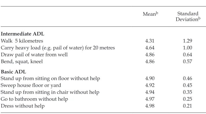
The ADL indices are calculated from responses to questions about nine daily physical activities (table 1). Answers to these questions are scored as follows: unable to do it (1); able to do it with dificulty (3); able to do it easily (5). The irst four of the nine ADLs listed in table 1 are used to calculate the intermediate ADL index, and the last ive are used for the basic ADL index. Again, the higher the value of the index, the better the presumed health status of the respondent.
Table 1 reports the mean and standard deviation of the results for each activity. These statistics are calculated for 4,132 household heads, using 2000 data only. As the table shows, the mean of each ADL is close to 5, implying that the vast major-ity of household heads can complete each task easily. However, the means of the irst four activities (the intermediate ADLs) are lower than those of the last ive
TABLE 1 Components of ADL Indicesa
Meanb Standard
Deviationb
Intermediate ADL
Walk 5 kilometres 4.31 1.29
Carry heavy load (e.g. pail of water) for 20 metres 4.64 1.00
Draw pail of water from well 4.86 0.64
Bend, squat, kneel 4.86 0.57
Basic ADL
Stand up from sitting on loor without help 4.90 0.46
Sweep house loor or yard 4.92 0.45
Stand up from sitting in chair without help 4.94 0.35
Go to bathroom without help 4.97 0.25
Dress without help 4.98 0.21
a The exact phrasing of the question on ADLs (activities of daily living) was as follows: ‘We would like
to know about your physical ability in daily activity. If you had to [do stated task], could you do it?’ The answer choices and corresponding scores were: ‘unable to do it’ (1); ‘able to do it with dificulty’ (3); and ‘able to do it easily’ (5). The sample size is 4,132 household heads.
b Means and standard deviations are calculated using data from the year 2000 only.
(the basic ADLs), implying that a larger proportion of household heads cannot easily perform the irst four tasks than is the case for the last ive. Accordingly, the standard deviations are larger for the irst four activities than for the last ive activities. It seems that capacity to perform the activities for the basic ADL index would be affected only by very severe physical limitations, while the intermediate ADL index would be sensitive to less serious limitations.
To calculate the ADL indices, we normalised the answers to each ADL question to the standard deviations from the mean; the indices are the means of the nor-malised scores for the relevant questions. For example, the mean and the standard deviation of ‘walk 5 kilometres’ are 4.31 and 1.29, respectively (table 1). The irst answer choice (‘unable to do it’) for this ADL is normalised as (1 – 4.31)/1.29, which is approximately –2.57. The intermediate ADL index is the arithmetic mean of the normalised values from the irst four ADL questions. A higher ADL index represents better health of the individual.
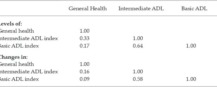
Table 2 presents simple pairwise correlations among our three health indicators – self-reported health, the intermediate ADL index and the basic ADL index – in terms of levels and changes, respectively. As can be seen in both parts of the table, the correlation between general health and each ADL index is low, implying that the measures of ADLs and general health capture different things. Further, the correlation between intermediate ADLs and basic ADLs is only 0.64 in the case of levels and 0.58 in the case of changes, suggesting that the two types of ADL indicators measure different dimensions of health.
Measurement of labour supply and consumption
Labour supply is measured in two ways: irst, whether the household head worked or not in the past year, and second, the number of hours worked by the household head in the past year. The IFLS collected information on household
TABLE 2 Pairwise Correlations between Health Measures in Terms of Levelsa and
Changesb
General Health Intermediate ADL Basic ADL
Levels of:
General health 1.00
Intermediate ADL index 0.33 1.00
Basic ADL index 0.17 0.64 1.00
Changes in:
General health 1.00
Intermediate ADL index 0.16 1.00
Basic ADL index 0.09 0.58 1.00
a The sample sizes for data on levels are 12,393 for column 1 and 12,396 for the other columns. The
same households are counted up to three times, in 1993, 1997 and 2000.
b The sample sizes for data on changes are 8,261 for column 1 and 8,264 for the other columns. The
same households are counted up to twice, relecting changes from 1993 to 1997 and from 1997 to 2000.
consumption using recall periods that differed for different consumption items. Information on food consumption, frequently purchased non-food items, and less frequently purchased non-food items was collected using recall periods of the past week, the past month and the past year, respectively.7 We calculate
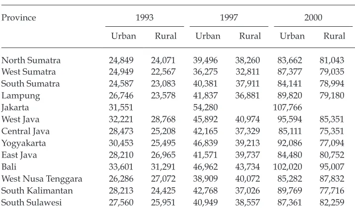
monthly per capita total non-medical consumption, which includes all kinds of food and non-food consumption excluding medical costs. We disaggregate non-medical consumption into two smaller categories: food consumption and non-food, non-medical consumption. We convert the nominal amounts of con-sumption into real terms using poverty lines proposed by Widyanti et al. (2009). Appendix table A1 lists the poverty lines for the 13 IFLS provinces, disaggre-gated into urban and rural areas. We use 2000 Jakarta prices (table A1) as the base.8 For example, suppose that a household in urban Bali had a nominal per
capita household food consumption of Rp 30,000 in 1993. The real per capita household food consumption of the same household using 2000 Jakarta prices as the base is 30,000 × 107,766 / 33,601, or Rp 96,217.
Descriptive statistics
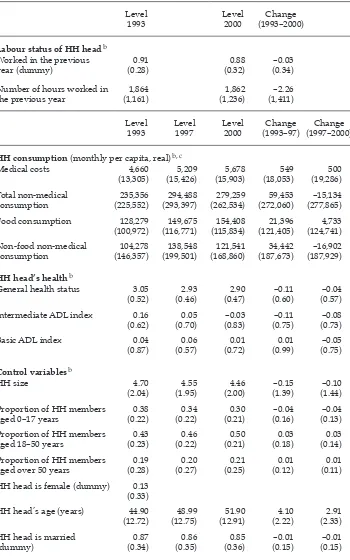
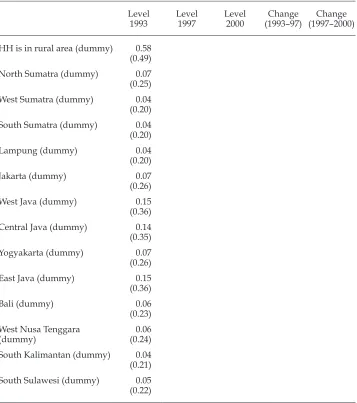
The means and standard deviations of household characteristics for the sample households used for regression analysis are reported in table 3. We provide the sample statistics not only in terms of levels but also in terms of changes, because the econometric identiication of our regressions comes from changes in health and changes in consumption or labour supply.
The means of the work (labour status) variables do not change much over time at the aggregate level, but the standard deviations of changes in the work variables over time are substantial. In fact, the standard deviations of the work variables are larger for changes in them than for their levels. For other vari-ables as well, including consumption and health, the standard deviations are in many cases larger for the changes than for the levels. For our regressions, we include these variables as change variables; their variations are substantial, as evidenced by the standard deviations of changes in these variables. For other variables such as household head’s age and marital status, the standard devia-tions are larger for the levels than for the changes. We use these variables, as well as the household head’s gender and the household’s location, as level vari-ables in our regressions.
7 Frequently purchased non-food items include utility services; household items such as soap and detergent; transport; and recreation. Less frequently purchased non-food items include clothing; furniture; and medical, education and ceremonial items and services. 8 By using 2000 Jakarta prices as the base (not only for Jakarta but for other regions as well), we generate real consumption igures that are comparable not only inter-temporally but also inter-regionally.
TABLE 3 Means and Standard Deviations of Household Characteristicsa
Level
1993 Level 2000 (1993–2000)Change
Labour status of HH headb
Worked in the previous
year (dummy) (0.28)0.91 (0.32)0.88 (0.34)–0.03 Number of hours worked in
the previous year (1,161)1,864 (1,236)1,862 (1,411)–2.26
Level
1993 Level 1997 Level 2000 (1993–97)Change (1997–2000)Change
HH consumption (monthly per capita, real)b, c
Medical costs 4,660
(13,305) (15,426)5,209 (15,903)5,678 (18,053)549 (19,286)500 Total non-medical
consumption (225,552)235,356 (293,397)294,488 (262,534)279,259 (272,060)59,453 (277,865) –15,134 Food consumption 128,279
(100,972) (116,771)149,675 (115,834)154,408 (121,405)21,396 (124,741)4,733 Non-food non-medical
consumption (146,357)104,278 (199,501)138,548 (168,860)121,541 (187,673)34,442 (187,929) –16,902
HH head’s healthb
General health status 3.05
(0.52) (0.46)2.93 (0.47)2.90 (0.60)–0.11 (0.57)–0.04 Intermediate ADL index 0.16
(0.62) (0.70)0.05 –0.03 (0.83) (0.75)–0.11 (0.73)–0.08
Basic ADL index 0.04
(0.87) (0.57)0.06 (0.72)0.01 (0.99)0.01 (0.75)–0.05
Control variablesb
HH size 4.70
(2.04) (1.95)4.55 (2.00)4.46 –0.15 (1.39) –0.10 (1.44) Proportion of HH members
aged 0–17 years (0.22)0.38 (0.22)0.34 (0.21)0.30 (0.16)–0.04 (0.13)–0.04 Proportion of HH members
aged 18–50 years (0.23)0.43 (0.22)0.46 (0.21)0.50 (0.18)0.03 (0.14)0.03 Proportion of HH members
aged over 50 years (0.28)0.19 (0.27)0.20 (0.25)0.21 (0.12)0.01 (0.11)0.01 HH head is female (dummy) 0.13
(0.33)
HH head’s age (years) 44.90
(12.72) (12.75)48.99 (12.91)51.90 (2.22)4.10 (2.33)2.91 HH head is married
(dummy) (0.34)0.87 (0.35)0.86 (0.36)0.85 (0.15)–0.01 (0.15)–0.01
TABLE 3 (continued) Means and Standard Deviations of Household Characteristicsa
Level
1993 Level 1997 Level 2000 (1993–97)Change (1997–2000)Change
HH is in rural area (dummy) 0.58
(0.49)
North Sumatra (dummy) 0.07
(0.25)
West Sumatra (dummy) 0.04
(0.20)
South Sumatra (dummy) 0.04
(0.20)
Lampung (dummy) 0.04
(0.20)
Jakarta (dummy) 0.07
(0.26)
West Java (dummy) 0.15
(0.36)
Central Java (dummy) 0.14
(0.35)
Yogyakarta (dummy) 0.07
(0.26)
East Java (dummy) 0.15
(0.36)
Bali (dummy) 0.06
(0.23)
West Nusa Tenggara
(dummy) (0.24)0.06
South Kalimantan (dummy) 0.04
(0.21)
South Sulawesi (dummy) 0.05
(0.22)
a Sample means and standard deviations for households (HH) used for the regressions are reported.
Sample standard deviations are in parentheses.
b The sample size for labour status of the HH head is 4,352 households. For almost all other variables,
the sample size is 4,132 households. HH head’s general health status and some consumption categories have slightly lower sample sizes for some years. For this reason the mean of the changes in these variables is not equal to the difference between the levels of the two means.
c Consumption data are in real per capita Rp/month at 2000 Jakarta prices.
ECONOMETRIC MODEL
Using the model developed by Gertler, Levine and Moretti (2003), we estimated the effect of health changes on changes in labour supply or household welfare (as proxied by consumption) in the following form:
ΔLit =α
jt+ β.ΔHit+δ.Xit+εit (1)
where the subscripts i, j and t indicate each household, region (either urban or rural area within a province) and year, respectively; ∆Litis the change in labour supply or per capita consumption of household
i
from year t–1 to year t (1993 to 2000 for labour supply and 1993 to 1997 or 1997 to 2000 for consumption); ∆Hitis the change in health status of household headi
from year t–1 to year t;9 and Xitis
the set of control variables described as follows:
• log initial (1993) real per capita household consumption; • log household size in year t–1;
• dummy for female-headed household in year t–1; • age of household head in year t–1;
• dummy for marital status of household head in year t–1; • change in log household size from year t–1 to year t;
• change from year t–1 to year t in the ratio of household members aged 0–17 to total household size; and
• change from year t–1 to year t in the ratio of household members aged 50 or older to total household size.
We further include a set of region–year dummies to control for region–year-speciic changes in the dependent variables – changes that were common across households within the same region–year.10 For example, economic growth was
faster in some regions than in others, and faster-growing regions may have experienced larger improvements (or reduced deteriorations) in health as a con-sequence of investing in medical facilities and equipment. These region–year dummies absorb differences in health-related investments across regions and years. Moreover, although we use real consumption as our dependent variable, conversion from nominal to real consumption is never perfect. The remaining differences in inlation across regions and years are also captured by these region– year dummies.11
9 One weakness of our study is that we do not take into account health shocks to productive household members other than household heads. If other working household members con-tribute signiicantly to household income, ignoring health shocks to them leads to imprecise estimates of the effect on household consumption of health shocks to household heads. 10 Both urban and rural areas exist in each of the 13 sample provinces except for Jakarta, where there are no rural areas, so there are 25 regions in the sample. We created region dummies for each change of years (the change from 1993 to 1997 and the change from 1997 to 2000). Thus, there are 50 region–year dummies. One of them, (urban) Jakarta from 1997 to 2000, is the reference group, so we include 49 region–year dummies in the regressions. Because of the inclusion of region–year dummies, the constant αjt is speciic for each re-gion–year.
11 Of course, the region–year dummies cannot address potential differences in omitted characteristics within region–years.
For regressions with consumption as the dependent variable, each sample household yields two observations (change from 1993 to 1997 and change from 1997 to 2000). We cluster standard errors at the household level to account for non-independence of the two observations from an identical household.12 Thus,
robust standard errors are unbiased in the presence of clusters at the household level and of any form of heteroscedasticity. For regressions with work as the dependent variable, each sample household yields only one observation, so we calculate the usual robust standard errors, which are unbiased in the presence of any form of heteroscedasticity.
The coeficient β is interpreted as the impact of household heads’ health changes on changes in household welfare. If households can perfectly insure their consumption against illness or injury suffered by household heads, β = 0.
We also estimate the following model to allow for differential health effects for farm and non-farm households:
ΔLit=αjt+ θ.FARM93
i+ β.ΔHit+γ.ΔHit.FARM93i+δ.Xit+εit (2)
This is the same as model (1) except for the two additional independent vari-ables: a dummy variable FARM93i and its interaction term with ∆Hit. The vari-able FARM93i takes the value 1 if at least one household member worked on a farm owned (at least partially) by the household in the past year as of 1993, and 0 otherwise. By interacting this dummy variable with changes in a health index, we can test whether the effect of health changes on labour hours or consumption is different in farm and non-farm households.
RESULTS AND DISCUSSION
Health shocks to household heads and changes in labour supply
Reduced work capacity of household heads is the main channel through which health shocks affect household consumption. In this section, we irst examine the extent to which health shocks lead to reduced labour supply by household heads.
Column 1 of table 4 presents the estimated effect of health changes on changes in the work participation of household heads. To save space, table 4 reports only the estimated coeficients on health changes and not those on the control variables mentioned in the previous section. We use changes in the various health measures (general health status, intermediate ADL index and basic ADL index) to explore the different degrees of sensitivity of labour supply to these concepts. We use a linear probability model where the dependent variable is change in work status
12 The ordinary least squares (OLS) technique implicitly assumes that sample observa-tions are randomly drawn from the population, implying that any observation should be a realisation from random sampling. In our case, however, a change in per capita house-hold expenditure is observed twice for each househouse-hold, both between 1993 and 1997 and between 1997 and 2000. These two observations for an identical household would not be two realisations from random sampling. For example, if the health of the household head deteriorated between 1993 and 1997, it is likely to have become even worse between 1997 and 2000. Because we have clustered standard errors at the household level, the resulting standard errors are unbiased, even if two observations from an identical household are not realisations from random sampling.
(the dummy variable is equal to 1 if the head worked in the previous year and 0 otherwise).13 Approximately 11% of observations have non-zero changes in work
status.
For both kinds of ADL indicators, the coeficient estimates on health changes are positive and statistically signiicant at the 1% level, while changes in general health status are not associated with changes in work participation at the con-ventional levels of signiicance. In terms of magnitude, a change in intermedi-ate ADLs has a larger estimintermedi-ated impact on labour force participation than does
13 A weakness of our study arises from the timing of the measurement of health status and labour supply. Health status was measured at the time of the survey interview, whereas labour supply was measured for the period one year before the date of the interview. Thus, our measures of labour supply are not sensitive to health shocks that occurred shortly before the date of the interview, especially in the case of the dummy for the household head’s participation in work. A similar weakness applies to our measures of household consumption.
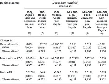
TABLE 4 Health Effects on Labour Supply and Household Consumptiona
Health Measure Dependent Variableb
General health 0.006 72.2** –1,033.0** 0.016 0.019 –0.001 status (0.009) (34.4) (454.8) (0.012) (0.013) (0.016) Observationsc 4,349 4,349 4,128 4,117 4,130 4,120
Intermediate ADL 0.068*** 94.2*** –1,395.4*** 0.029*** 0.032*** 0.018 (0.009) (25.1) (487.9) (0.011) (0.012) (0.013) Observationsc 4,352 4,352 4,130 4,119 4,132 4,122
Basic ADL 0.025*** 14.9 –534.8 0.017** 0.018* 0.015 (0.007) (18.3) (396.9) (0.008) (0.009) (0.011) Observationsc 4,352 4,352 4,130 4,119 4,132 4,122
a Robust standard errors are shown in parentheses. In columns 1–2, robust standard errors are
unbiased in the presence of any form of heteroscedasticity. In columns 3–6, robust standard errors are unbiased in the presence of clusters at the household level and of any form of heteroscedasticity. *** signiicant at 1%; ** signiicant at 5%; * signiicant at 10%.
b Columns 3–6 are based on expenditure in real per capita Rp/month at 2000 Jakarta prices. c The number of sample households is reported for each regression.
a change in basic ADLs. For example, the estimated coeficient on intermediate ADLs implies that a 1 standard deviation (SD) increase in intermediate ADLs is associated with approximately a 7 percentage point increase in the probability of working. By comparison, a 1 SD increase in basic ADLs results in a less than 3 percentage point increase in the probability of working.14 We ind the strongest
statistical association between labour participation and intermediate ADLs, pos-sibly because the activities used to calculate the intermediate ADL index are more relevant for work participation than those used to calculate the basic ADL index.
Column 2 of table 4 presents the estimated effect of health changes on changes in labour hours worked by household heads in the past year. Health changes are positively and signiicantly correlated with changes in work hours, except in the case where the basic ADL index is used as the health indicator. We ind a positive and statistically signiicant association between self-reported general health and work hours. This could be due partly to the effect of health on work hours and partly to the justiication of reduced work hours discussed by Bound (1991) and mentioned in the introduction: those who are not working or have reduced their work hours tend to report worse health to justify this. Again, activities included in the intermediate ADL index could be most relevant to work hours, since we ind the strongest statistical correlation between health changes and work hours when we use intermediate ADLs as the health measure. A 1 SD increase in intermediate ADLs is associated with an additional 94 work hours per year.
Health shocks to household heads and changes in household consumption
Column 3 of table 4 shows the estimated effect of changes in health on changes in monthly medical expenditures. Because many sample households report zero medical expenses in some or all sample years, we use changes in real per capita medical expenditures without taking logarithms for the dependent variable.15
We ind strong associations between changes in health and changes in medical expenditures except for the case where the basic ADL index is used as the health measure. In terms of magnitude, a 1 SD increase in intermediate ADLs reduces monthly expenditure on medical costs by Rp 1,395, or approximately 25% of mean monthly real per capita medical costs (Rp 5,678) in 2000 (table 3). Household med-ical expenditure is also responsive to changes in self-reported general health. A one-category improvement (say, from ‘reasonably healthy’ to ‘very healthy’) in self-reported general health reduces monthly per capita medical expenditure by Rp 1,033, or approximately 18% of mean monthly real per capita medical costs. The degree of correlation between medical costs and the basic ADL index is weak. A low basic ADL index implies serious physical disability. It is possible that households strategically spend more money on medical treatment for household
14 Strictly speaking, a 1 SD decrease in intermediate ADLs is not comparable with a 1 SD decrease in basic ADLs. Thus, the magnitudes of the coeficient estimates on the ADL in-dices should be interpreted with caution. However, the degree of statistical correlation be-tween the dependent variable and each ADL index should be useful in determining which kinds of daily activities move more closely together with the dependent variable (labour supply in this sub-section and household consumption in the next sub-section).
15 Since the logarithm of 0 is undeined, relying on the logarithm of real per capita medical expenditure would reduce the number of sample households by about 30%.
heads who are mildly ill or injured (and hence have a high probability of regain-ing labour productivity) than for household heads who are severely ill or injured (and have little or no hope of regaining labour productivity).
Columns 4–6 of table 4 use changes in log per capita non-medical consump-tion, changes in log per capita food consumption and changes in log per capita non-food, non-medical consumption as the dependent variable, respectively. Our indings are as follows. First, self-reported general health has no statistically sig-niicant correlation with any of the three consumption categories. This inding may not be surprising, given the very subjective nature of self-reported general health status as a health measure. Second, each ADL indicator has positive correla-tions with both non-medical consumption and food consumption at conventional levels of signiicance. The magnitude of the association between consumption and health is larger for intermediate ADLs (about 0.03) than for basic ADLs (about 0.02). However, the results suggest that the effect of health on consumption may not be large. For example, a 1 SD increase in intermediate ADLs is associated with an increase in food consumption of only about 3%. Third, the association between non-food, non-medical consumption and each of the ADL indicators is even smaller, and no correlation is statistically signiicant.
These indings imply that if changes in the household head’s health are serious enough to inluence his or her ADLs, household consumption will be only slightly affected, suggesting that household consumption is largely protected – probably by formal and informal risk-coping mechanisms. Most notably, other household members may increase labour supply in response to adverse health shocks to household heads. The estimation result implies that even if the intermediate ADL index of a household head deteriorates by 2 SDs, household food consumption will decline by only 6%.
A plausible explanation for our inding that changes in intermediate ADLs have a stronger inluence on labour supply and household consumption than changes in basic ADLs is as follows. Initial health status may already be low for those who later experience health shocks serious enough to affect basic ADLs, so the contributions of such household heads to household incomes could be low
TABLE 5 Work Hours in 1992 for Household Heads With and Without Later Health Shocksa
Change in ADL between 1993 and 2000 No Change in ADL
(Change = 0) ADL Deteriorated (Change < 0)
Intermediate ADL N = 3,028 N = 1,047
Median work hours in 1992 1,960 (100%) 1,536 (78%)
Basic ADL N = 3,986 N = 243
Median work hours in 1992 1,872 (96%) 910 (46%)
a Percentages are of the median work hours of those who later (between 1993 and 2000) experienced
no negative change in intermediate ADL (1,960 hours).
in the irst place (no matter whether they experience health shocks later or not). However, for household heads who later experience health shocks that affect only intermediate ADLs, this may not be the case.
Table 5 provides median work hours as of 1992 separately for household heads who later experienced adverse health shocks and for those who did not. We do this using the same two deinitions of health shocks – negative changes in inter-mediate ADLs, and negative changes in basic ADLs. Median work hours as of 1992 were 1,960 for those who later experienced no change in intermediate ADLs between 1993 and 2000. Median work hours as of 1992 were 1,536 (78% of 1,960) for those who later experienced negative changes in intermediate ADLs, but only 910 (46% of 1,960) for those who later experienced negative changes in basic ADLs. Clearly, work hours as of 1992 were already lower for household heads who later experienced negative changes in basic ADLs. This is consistent with our inter-pretation that if household heads later experienced such a serious health shock as to affect basic ADLs, their initial work hours were probably already low, so health shocks may not have affected their work hours and household consump-tion as much as health shocks to household heads whose intermediate ADLs were damaged.16
Our results may look odd if food consumption is considered as more of neces-sity than non-food consumption, because demand for necessities is less income-elastic than that for less necessary items. In examining the economic consequences of health shocks using Vietnamese data, Wagstaff (2007) inds that households spend less on food following a health shock but spend more on budget items such as housing and electricity – probably to accommodate the needs of the ill or injured household members. Our own econometric analysis suggests that house-hold food consumption on average seems to be reasonably well protected against health shocks to household heads. Given that demand for food is mostly satisied, it is plausible that some households spend on non-food items such as housing and electricity that may assist the recovery of the ill or injured, by reducing consump-tion of other non-food items that are luxuries by nature, such as leisure. The net effect of changes in food purchases could make household food, non-medical consumption less responsive to health shocks. Alternatively, measure-ment errors may be more severe for non-food items than for food items because of the longer recall periods used for them in the surveys. Further, it is possible that our health indicators (which measure health status at the time of the survey inter-views) are more strongly correlated with recent consumption (food consumption with a one-week recall period) than with distant consumption (non-food items with either one-month or one-year recall periods). To explore these possibilities
16 Table 5 conirms the validity of our econometric identiication strategy. It supports the conjecture that poor or unhealthy household heads are more likely to experience nega-tive health shocks than those in better health or inancial circumstances. In other words, household heads who later experience adverse health shocks during a given period of time are on average already less healthy or poorer than household heads who do not later experience adverse health shocks. If the level of household consumption is regressed on indicators of adverse health shocks, such as a sizeable decline in BMI or a long in-patient spell (as in Wagstaff 2007), the estimation would be biased, because households that later experience adverse health shocks tend to be relatively unhealthy and poor to begin with.
further, it would be necessary to analyse the relationships between health shocks and more disaggregated consumption categories.
The coeficient estimates on the main statistically signiicant control variables (not shown in table 4) can be summarised briely as follows.17 First, low levels of
per capita household expenditure as of 1993 are associated with higher percent-age increases in per capita household expenditures. Second, female household headship is associated with lower percentage increases in per capita household expenditures. Third, older age of the household head is associated with lower percentage increases in per capita household expenditures. Fourth, both larger lagged household size and larger changes in household size are associated with smaller elasticities with respect to increases in per capita household expenditures. Fifth, negative changes in the share of the age group 0–17 in households are asso-ciated with higher percentage increases in both per capita food expenditure and per capita total non-medical expenditure, but this coeficient estimate is not sta-tistically signiicant when per capita non-medical, non-food expenditure is used as the dependent variable.
Health shock effects on welfare of farm and non-farm households
Farming is a physically demanding job. If health shocks to household heads are so severe as to affect their ADLs, such health shocks may reduce the work potential of farmers to a more serious extent than that of household heads whose jobs are more sedentary. Accordingly, household consumption could deteriorate more in farm households than in non-farm households following a health shock. In this section, we test the hypothesis that farm households are less well protected than non-farm households against adverse health shocks.
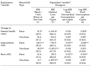
Our results from estimating 12 different versions of model (2) above are con-tained in table 6. Four dependent variables are used in the regression: changes in labour hours worked by household heads (column 1); changes in per capita medi-cal consumption (column 2); changes in log per capita total non-medimedi-cal consump-tion (column 3); and changes in log per capita food consumpconsump-tion (column 4). The same set of control variables is used as before (but, to save space, their coeficient estimates are not reported). The coeficient estimates for farm households reported in table 6 are the sums of the two coeficient estimates (β + γ) in model (2).18
As seen in column 1, the impact of a health shock on labour hours worked by the household head seems to be stronger in farm than in non-farm households, regardless of which health measure is used. However, labour hours of non-farm household heads still seem to be quite responsive to changes in intermediate ADLs. In response to a 1 SD decrease in intermediate ADLs, farm and non-farm household heads reduce their yearly work hours by 100 and 88 hours, respectively.
17 The coeficient estimates on the control variables are similar, regardless of the catego-ries of consumption and the measures of health.
18 The estimated value of θ in model (2) is statistically signiicant at conventional levels only when the dependent variable is either food consumption or total non-medical con-sumption (no matter which health measure is used). For both types of concon-sumption the estimated value of θ is positive, implying that farm households on average increased (re-duced) food consumption and total non-medical consumption proportionately more (less) than non-farm households.
Broadly speaking, column 2 shows the expected negative relationship between medical costs and health. Nevertheless, the result is quite different depending on whether the independent variable is self-reported general health status or one of the ADL measures. Per capita medical costs are far more strongly affected by ADL health shocks in non-farm than in farm households, while the opposite is true if self-reported general health is used as the health measure (though the coeficient for farm households is only weakly signiicant). It could be that farm households do not use medical care as much as non-farm households do for health shocks that are serious enough to affect daily activities, but may do so as much as or perhaps more than non-farm households for less severe symptoms. This potential difference in medical care use between farm and non-farm households could be due to supply-side conditions: rural areas may provide only primary care,
TABLE 6 Different Effects for Farm and Non-Farm Householdsa
Explanatory
Variable Household Type Dependent Variable
b
status Farm (49.5)91.9* –1,169.6*(640.1) (0.019)0.026 (0.021)0.035*
Non-farm 55.4 –916.5 0.007 0.005
(47.2) (631.0) (0.015) (0.016) Intermediate
ADL Farm (35.5)100.1*** (683.1)–706.9 (0.015)0.037** (0.015)0.044*** Non-farm 88.0*** –2,100.1*** 0.019 0.019
(33.3) (672.5) (0.015) (0.018)
Basic ADL Farm 32.4 233.3 0.027** 0.026**
(22.1) (484.8) (0.012) (0.013)
Non-farm –8.7 –1,499.0** 0.003 0.007
(30.5) (584.9) (0.011) (0.014)
aRobust standard errors are in parentheses.
In the irst column, robust standard errors are unbiased in the presence of any form of heteroscedastic-ity. In the remaining columns, robust standard errors are unbiased in the presence of clusters at the household level and of any form of heteroscedasticity.
The covariates include a dummy for farm households; log initial (1993) level of per capita total con-sumption; change in log household size; lagged log household size; change in proportion of house-hold members aged 0–17; change in proportion of househouse-hold members aged 50 or older; househouse-hold head’s gender, age and marital status; and 49 region–year dummies.
The number of sample households varies between 4,117 and 4,352. *** signiicant at 1%; ** signiicant at 5%; * signiicant at 10%.
b Columns 2–4 are based on expenditure in real per capita Rp/month at 2000 Jakarta prices.
whereas urban areas have medical facilities to provide more advanced care. Our results with the ADL indices suggest dramatically different responses to health shocks by the two groups of households: non-farm households clearly increase their spending on medical care, whereas there is no evidence that farm house-holds do so.
The results in column 3 suggest that total non-medical consumption is inlu-enced by health shocks only in farm households. For example, in response to a 1 SD decrease in intermediate ADLs, farm households reduce their total non-medical consumption by 4%; by comparison, none of the coeficients for non-farm households is signiicantly different from zero.
In column 4, the association between health changes and changes in food con-sumption is statistically signiicant only for farm households. In terms of the mag-nitudes of the coeficient estimates, column 4 is similar to column 3. For example, a 1 SD decrease in intermediate ADLs reduces farm households’ food consump-tion by 4% on average.
If we use changes in log per capita non-food, non-medical consumption as the dependent variable (not reported in table 6), no coeficient estimate on health changes is statistically different from zero for either farm or non-farm households, regardless of which health indicator is used.
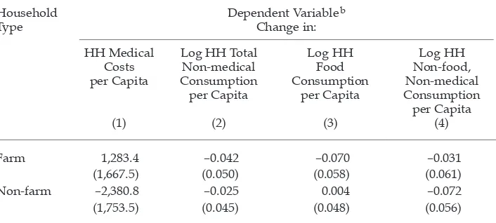
Finally, we briely examine the death of a household head as a health shock measure. The death of the household head is in a sense the most extreme health shock to a household (although its impact on household per capita consumption may well be less than would be the case if the household head became incapaci-tated). The IFLS identiies deaths of household heads that occurred between the surveys. We use a dummy for death equal to unity for 1997 if the household head died between 1993 and 1997, and equal to zero otherwise. Similarly, we use a dummy for death equal to unity for 2000 if the household head died between 1997 and 2000, and equal to zero otherwise. We estimated model (2) using the dummy for death of a household head as the health measure. The results are reported in appendix table A2, whose structure is similar to that of table 6. The depend-ent variables used in table A2 are changes in per capita medical consumption (column 1); changes in log per capita total non-medical consumption (column 2); changes in log per capita food consumption (column 3); and changes in log per capita non-food, non-medical consumption (column 4). Table A2 reports the results from four separate regressions.
Because the death dummy is unity for only 4% of observations, the standard errors of the coeficient estimates are large. Thus, none of the coeficient estimates on the death dummy is statistically signiicant at conventional levels of signii-cance. However, it seems that our earlier indings regarding differences in farm and non-farm households are supported: total non-medical consumption and food consumption are more strongly affected by health shocks in farm house-holds than in non-farm househouse-holds, and medical costs are more responsive to health shocks in non-farm households than in farm households.19
19 Column 1 of table A2 suggests that after the deaths of the household heads, medical costs decline in non-farm households but increase in farm households, but neither effect is statistically signiicant.
Our indings in this section are consistent with the hypothesis that farmers are more vulnerable to health shocks in terms of labour supply and household total non-medical consumption and food consumption.
CONCLUSION
This paper is concerned with the effect on household welfare of a health shock to the household head. We are particularly interested in whether household con-sumption is protected against major illness or injury shocks to household heads. To examine this question, we use ADL indices as measures of health that are sen-sitive to major illness or injury shocks. We also use multiple consumption cat-egories to examine the differential effects of health changes on different types of consumption. Further, we use changes in consumption or labour supply and changes in health measures for the econometric identiication to control for all time-invariant characteristics that may bias our results.
Our results still may be biased owing to the potential presence of omitted time-varying characteristics that are correlated with both changes in labour supply or consumption and changes in health. With this caveat in mind, our indings are as follows.
First, labour supply and household consumption are more responsive to the intermediate ADL index than to the basic ADL index.20 We believe that the
activi-ties represented by the intermediate ADL index are the most relevant as measures of the work potential of household heads over the sample period. In this respect, our results provide a stark contrast to those of Gertler and Gruber (2002), who found that household consumption was more sensitive to their basic ADL index. In their study, the sample households were selected from two provinces only (West Nusa Tenggara and East Kalimantan) in 1991 and 1993, while our sample households were chosen from 13 provinces in 1993, 1997 and 2000. The difference in sample sites and timing may explain the different results.21
Second, major illness and injury shocks (to the extent that they affect intermedi-ate ADLs) would be expected to affect labour supply by household heads as well as household consumption behaviour. However, the consumption of Indonesian households seems typically to be well protected against health shocks. A quite
20 Our argument is based on the degree of statistical correlation between the dependent variable (labour supply or household consumption) and each of the ADL indices.
21 Gertler and Gruber (2002) examined the effect of ADL changes on changes in labour supply using the overall ADL index only (that is, with no separate estimation for interme-diate and basic ADL changes). They used intermeinterme-diate and basic ADL changes separately as the instrument for changes in income in estimating the effect of income changes on expenditure changes. Since they imputed wages to all workers based on wages in the for-mal labour market (no matter whether each sample household head worked in the forfor-mal labour market or in a family farm or enterprise), their income imputation, which is the product of the imputed wages and labour-supply hours, ignored the effect of health shocks on the returns to labour, as the authors acknowledge on page 57 of their paper. If interme-diate ADL shocks have a larger effect on the return to labour than basic ADL shocks, then Gertler and Gruber (2002) under-estimate the importance of intermediate ADLs relative to basic ADLs in their estimation of the effect of ADL changes on changes in household expenditure through changes in household income.
large health shock, such as a 1 SD decrease in intermediate ADLs, reduces the household’s total consumption and food consumption by only 3% on average, implying the presence of formal and/or informal risk-coping mechanisms.22 Our
indings are therefore consistent with the economic literature on consumption insurance long studied by economists (Townsend 1995).
Third, we ind that farm households are more inluenced by health shocks than non-farm households in terms of both hours of work by household heads and household food consumption. However, even farmers seem to be quite well pro-tected against health shocks. A 1 SD decrease in intermediate ADLs reduces food consumption by only 4% on average in farm households.
Finally, we ind another potentially important difference between farm and non-farm households in terms of response behaviour to health shocks. Non-farm households are much more responsive to health shocks than farm households in terms of household medical consumption. It is not clear whether this is because of low demand for medical care among farmers even in the face of health shocks, or because of low availability of medical services in rural areas. In either case, fac-tors other than household inancial resources may affect farmers’ use of medical services.
Overall, our indings point to the presence of well-functioning risk-coping mechanisms over the sample period. Thus, establishment of public risk-coping systems against health shocks, such as public disability insurance and subsidies for medical care, may not be a pressing need for typical Indonesian households. However, our study has not addressed how people cope with health shocks. It could be that children are forced to discontinue their education because of the need to work in response to adverse health shocks to household heads. Alter-natively, it may be that household savings can support living standards only for a short period, while the disability of a household head could persist for much longer. To evaluate the desirability of establishing public risk-coping systems against health shocks, further studies would be necessary, focusing on how peo-ple cope with health shocks, the longer-term impact of health shocks on house-hold welfare, and the impact of health shocks on more disaggregated househouse-hold consumption (to determine what kinds of non-food consumption are responsive and not responsive to health shocks).
22 The present study did not examine the impact of a large health shock (such as a 1 SD decrease in intermediate ADLs) on household income. Thus it is possible that a 1 SD de-crease in intermediate ADLs reduces household income (and consumption) by only 3%, which would imply the absence of any risk-coping (consumption insurance) mechanism. However, given the nature of the ADL indices, it seems implausible that a 1 SD decrease in intermediate ADLs would have so little impact on household income.
REFERENCES
Bound, John (1991) ‘Self-reported versus objective measures of health in retirement mod-els’, Journal of Human Resources 26 (1): 106–38.
Christiaensen, Luc, Hoffmann, Vivian and Sarris, Alexander (2007) ‘Gauging the welfare effects of shocks in rural Tanzania’, Policy Research Working Paper 4406, World Bank, Washington DC.
Dercon, Stefan (2003) ‘Insurance against poverty’, Policy Brief, United Nations University, Tokyo.
Dercon, Stefan, Hoddinott, John and Woldehanna, Tassew (2005) ‘Shocks and consumption in 15 Ethiopian villages, 1999–2004’, Journal of African Economies 14 (4): 559–85.
Gertler, Paul and Gruber, Jonathan (2002) ‘Insuring consumption against illness’, American Economic Review 92 (1): 51–70.
Gertler, Paul, Levine, David I. and Moretti, Enrico (2003) ‘Do microinance programs help families insure consumption against illness?’, Working Paper Series 1045, Center for International and Development Economics Research, Institute for Business and Eco-nomic Research, University of California, Berkeley CA.
Hoogeveen, Johannes, Tesliuc, Emil and Vakis, Renos with Dercon, Stefan (2004) ‘A guide to the analysis of risk, vulnerability and vulnerable groups’, World Bank, Washington DC.
Lindelow, Magnus and Wagstaff, Adam (2005) ‘Health shocks in China: are the poor and uninsured less protected?’, Policy Research Working Paper 3740, World Bank, Wash-ington DC.
McDowell, Ian (2006) Measuring Health: A Guide to Rating Scales and Questionnaires, 3rd ed., Oxford University Press, New York NY.
Prescott, Nicholas and Pradhan, Menno (1999) Coping with catastrophic health shocks, Paper presented at a conference on ‘Social Protection and Poverty’, Inter-American Development Bank, Washington DC, 5 February.
Strauss, John, Gertler, Paul J., Rahman, Omar and Fox, Kristin (1993) ‘Gender and life-cycle differentials in the patterns and determinants of adult health’, Journal of Human Resources 28 (4): 791–837.
Strauss, John, Beegle, Kathleen, Sikoki, Bondan, Dwiyanto, Agus, Herawati, Yulia and Witoelar, Firman (2004) The Third Wave of the Indonesia Family Life Survey: Overview and Field Report, Volume 1, RAND Corporation, Santa Monica CA.
Strauss, John and Thomas, Duncan (1998) ‘Health, nutrition, and economic development’, Journal of Economic Literature 36 (2): 766–817.
Thomas, Duncan and Strauss, John (1997) ‘Health and wages: evidence on men and women in urban Brazil’, Journal of Econometrics 77 (1): 159–85.
Townsend, Robert M. (1995) ‘Consumption insurance: an evaluation of risk-bearing sys-tems in low-income economies’, Journal of Economic Perspectives 9 (3): 83–102.
Wagstaff, Adam (2007) ‘The economic consequences of health shocks: evidence from Viet-nam’, Journal of Health Economics 26 (1): 82–100.
Widyanti, Wenefrida, Suryahadi, Asep, Sumarto, Sudarno and Yumna, Athia (2009) ‘The relationship between chronic poverty and household dynamics: evidence from Indo-nesia’, SMERU Working Paper No. 132, SMERU Research Institue, Jakarta.
Yagura, Kenjiro (2005) ‘Why illness causes more serious economic damage than crop fail-ure in rural Cambodia’, Development and Change 36 (4): 759–83.
APPENDIX
TABLE A1 Poverty Lines for 1993, 1997 and 2000 (Rp per capita per month)
Province 1993 1997 2000
Urban Rural Urban Rural Urban Rural
North Sumatra 24,849 24,071 39,496 38,260 83,662 81,043 West Sumatra 24,949 22,567 36,275 32,811 87,377 79,035 South Sumatra 24,587 23,083 40,381 37,911 84,141 78,994 Lampung 26,746 23,578 41,837 36,881 89,820 79,180
Jakarta 31,551 54,280 107,766
West Java 32,221 28,768 45,892 40,974 95,594 85,351 Central Java 28,473 25,208 42,165 37,329 85,111 75,351 Yogyakarta 30,453 25,495 46,839 39,213 92,086 77,094 East Java 28,210 26,965 41,571 39,737 84,480 80,752
Bali 33,601 31,291 46,962 43,734 102,020 95,007
West Nusa Tenggara 26,286 27,072 38,909 40,072 85,282 87,832 South Kalimantan 28,213 24,425 42,768 37,026 89,769 77,716 South Sulawesi 27,560 25,951 40,949 38,557 87,361 82,259
Source: Widyanti et al. (2009).
TABLE A2 Effects of Household Head’s Death on Household Consumptiona
Household
Type Dependent Variable
b
Change in: HH Medical
Costs per Capita
(1)
Log HH Total Non-medical Consumption
per Capita
(2)
Log HH Food Consumption
per Capita
(3)
Log HH Non-food, Non-medical Consumption
per Capita (4)
Farm 1,283.4 –0.042 –0.070 –0.031
(1,667.5) (0.050) (0.058) (0.061)
Non-farm –2,380.8 –0.025 0.004 –0.072
(1,753.5) (0.045) (0.048) (0.056)
a Robust standard errors are in parentheses.
Robust standard errors are unbiased in the presence of clusters at the household level and of any form of heteroscedasticity.
No estimated coeficient is statistically signiicant.
The covariates include a dummy for farm households; log initial (1993) level of per capita total con-sumption; change in log household size; lagged log household size; change in proportion of household members aged 0–17; change in proportion of household members aged 50 or older; and 49 region–year dummies.
The number of sample households varies between 5,933 and 5,955.
The number of sample households differs between this table and table 6 mainly because table 6 does not use the following sample households:
• those for which ADLs of household heads are not reported; and
• those that experienced a change in household head for whatever reason, including the death of the household head.
b Columns 1–4 are based on expenditure in real per capita Rp/month at 2000 Jakarta prices.