Full Terms & Conditions of access and use can be found at
http://www.tandfonline.com/action/journalInformation?journalCode=ubes20
Download by: [Universitas Maritim Raja Ali Haji] Date: 11 January 2016, At: 22:26
Journal of Business & Economic Statistics
ISSN: 0735-0015 (Print) 1537-2707 (Online) Journal homepage: http://www.tandfonline.com/loi/ubes20
Comment
Barbara Rossi
To cite this article: Barbara Rossi (2012) Comment, Journal of Business & Economic Statistics, 30:1, 25-29, DOI: 10.1080/07350015.2012.634343
To link to this article: http://dx.doi.org/10.1080/07350015.2012.634343
Published online: 22 Feb 2012.
Submit your article to this journal
Article views: 112
4. CONCLUSION
I find the ideas put forward in this article to rigorously test the optimality of forecasts across horizons interesting and the efforts to implement the tests quite commendable. Despite their math-ematical elegance, these derived bounds are implied by forecast rationality, and hence are not necessary conditions. Thus, if the tests do not reject the null, we cannot say we have evidence in favor of rationality. For instance, even though the forecast vari-ances and MSEs are observed to be weakly decreasing functions of the forecast horizon, the underlying forecasts can be easily be still inefficient. By using Blue Chip and SPF survey fore-casts, we found, like PT, that some of the bounds tests proposed in the paper are not very powerful to detect suboptimality in instances where the extant Nordhaus test readily identifies it. However, their new extended MZ test based on a regression of the target variable on the long-horizon forecast and the se-quence of interim forecast revisions works well, provided the multicollinearity problem does not become serious. We have argued that by testing the equality of MSE differentials with mean square forecast revisions, one can also examine forecast rationality over multiple horizons. In order to truly understand the pathways through which forecasts fail to satisfy forecast op-timality, we have also to consider the demand side of the fore-casting market and the schedule of official data announcements. For instance, there is evidence that forecasters record maximum suboptimality at horizons where they also make maximum cast revisions. The observed suboptimality of Greenbook fore-casts that PT found cannot be understood unless the institu-tional requirements of such forecast are appreciated. Neverthe-less, the importance of testing the joint implications of forecast
rationality across multiple horizons when such information is available as proposed by the authors must be appreciated.
ACKNOWLEDGMENTS
The author thanks Antony Davies, Gultikin Isiklar, Huaming Peng, Xuguang Sheng, and Yongchen Zhao for many useful discussions and research assistance, and to the co-editors for making a number of helpful comments.
[Received June 2011. Revised July 2011.]
REFERENCES
Clements, C. P., Joutz, F., and Stekler, H. (2007), “An Evaluation of Forecasts of the Federal Reserve: A Pooled Approach,”Journal of Applied Econometrics, 22, 121–136. [24]
Davies, A., and Lahiri, K. (1999), “Re-examining the Rational Expectations Hypothesis Using Panel Data on Multi-period Forecasts,” in Analysis of Panels and Limited Dependent Variables, eds. C. Hsiao, K. Lahiri, L. F. Lee, and H. Pesaran, Cambridge, U.K.: Cambridge University Press, pp. 226–254. [22]
Isiklar, G., and Lahiri, K. (2007), “How Far Ahead can We Forecast? Evidence from Cross-country Surveys,”International Journal of Forecasting, 23, 167– 187. [21,22]
Lahiri, K., and Sheng, X. (2008), “Evolution of Forecast Disagreement in a Bayesian Learning Model,”Journal of Econometrics, 144, 325–340. [23,24] Lahiri, K., and Sheng, X. (2010), “Learning and Heterogeneity in GDP and Inflation Forecasts,” International Journal of Forecasting, 26, 265– 292. [24]
Mankiw, N. G., and Shapiro, M. D. (1986), “News or Noise? An Analysis of GNP Revisions,”Survey of Current Business, 66, 20–25. [21]
Nordhaus, W. (1987), Forecasting Efficiency; Concepts and Applications, Re-view of Economics and Statistics, 69, 667–674. [22]
Comment
Barbara R
OSSIDepartment of Economics, 204 Social Science Building, Duke University, Durham, NC 27708, ICREA, and University Pompeu ([email protected])
Patton and Timmermann (2011) propose new and creative forecast rationality tests based on multi-horizon restrictions. The novelty is to consider the implications of forecast rationality jointly across the horizons. They focus on testing implications of forecast rationality such as the fact that the mean squared forecast error should be increasing with the forecast horizon (Diebold 2001; Patton and Timmermann 2007) and that the mean squared forecast should be decreasing with the horizon. They also consider new regression tests of forecast rationality that use the complete set of forecasts across all horizons in a univariate regression, which they refer to as the “optimal revi-sion regresrevi-sion” tests. One of the advantages of the proposed procedures is that they do not require researchers to observe the target variable, which sometimes is not clearly available. In fact, Patton and Timmermann (2011) show that both their in-equality results as well as the “optimal revision regression” test hold when the short horizon forecast is used in place of the target variable. Their work is an excellent contribution to the literature.
The main objective of this comment is to check the robust-ness of forecast rationality tests to the presence of instabilities. The existence of instabilities in the relative forecasting perfor-mance of competing models is well known [see Giacomini and Rossi (2010) and Rossi and Sekhposyan (2010), among others; Rossi (2011) provide a survey of the existing literature on forecasting in unstable environments]. First, we show heuris-tic empirical evidence of time variation in the rolling estimates of the coefficients of forecast rationality regressions. We then use fluctuation rationality tests, proposed by Rossi and Sekh-posyan (2011), to test for forecast rationality, while, at the same time, being robust to instabilities. We also consider a version of Patton and Timmermann’s (2010) optimal revision
© 2012American Statistical Association Journal of Business & Economic Statistics
January 2012, Vol. 30, No. 1 DOI:10.1080/07350015.2012.634343
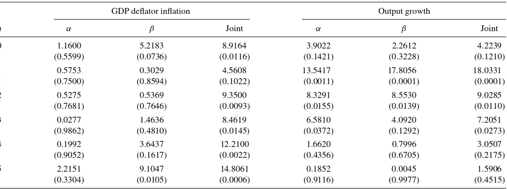
Table 1. Full-sample Mincer and Zarnowitz (1969) forecast rationality tests
GDP deflator inflation Output growth
h α β Joint α β Joint
0 1.1600 5.2183 8.9164 3.9022 2.2612 4.2239
(0.5599) (0.0736) (0.0116) (0.1421) (0.3228) (0.1210)
1 0.5753 0.3029 4.5608 13.5417 17.8056 18.0331
(0.7500) (0.8594) (0.1022) (0.0011) (0.0001) (0.0001)
2 0.5275 0.5369 9.3500 8.3291 8.5530 9.0285
(0.7681) (0.7646) (0.0093) (0.0155) (0.0139) (0.0110)
3 0.0277 1.4636 8.4619 6.5810 4.0920 7.2051
(0.9862) (0.4810) (0.0145) (0.0372) (0.1292) (0.0273)
4 0.1992 3.6437 12.2100 1.6620 0.7996 3.0507
(0.9052) (0.1617) (0.0022) (0.4356) (0.6705) (0.2175)
5 2.2151 9.1047 14.8061 0.1852 0.0045 1.5906
(0.3304) (0.0105) (0.0006) (0.9116) (0.9977) (0.4515)
NOTE: Full-sample Mincer and Zarnowitz (1969) regression, Equation (1).P-values based on HAC robust estimates (with bandwidth equal to 3) for testingα=0 (column labeled “α”), β=1 (column labeled “β”), and bothα=0 andβ=1 (column labeled “Joint”) in parentheses.
regression test robust to instabilities, which we will refer to as the “fluctuation revision” test. Finally, we discuss the empirical evidence.
We focus on the same data as in Patton and Timmermann (2010), which include the Federal Reserve “Greenbook” fore-casts of quarter-over-quarter rates of change in GDP and the GDP deflator. The data are from Faust and Wright (2009), start-ing in 1980 and endstart-ing in 2002.
First, we consider the typical “full-sample” Mincer and Zarnowitz (1969) forecast rationality test. Let the target value to be forecasted at time t using information up to timet−h beytand let the forecast be denoted byyt|t−h. The Mincer and Zarnowitz (1969) regression is as follows:
yt =α+βyt|t−h+εt,h, t =1, . . . , P , (1)
where P is the number of out-of-sample forecasts, h is the forecast horizon, and εt,h is the residual. If the forecasts are unbiased, the constantαshould be statistically insignificantly different from zero; if the forecasts are optimal, the slope β should be statistically insignificantly different from unity. The null hypothesis of forecast rationality is thatα=0 andβ =1, jointly.Table 1reports the results. The table shows that forecast rationality is rejected at the 5% significance level for the GDP deflator inflation at most horizons, and it is rejected at horizons 1–3 for GDP growth.
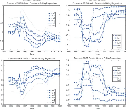
However, the estimates of αandβ may not be stable over time. The presence of instability is a serious concern, since it would imply that typical forecast rationality tests are invalid. See Rossi (2005) for an intuitive discussion of why full-sample tests are invalid in the presence of instabilities. To provide in-formal evidence,Figure 1reports estimates ofαandβin rolling regressions, using a window of 60 out-of-sample forecast obser-vations. Thex-axis is the time of the latest forecast included in the rolling regression sample.Figure 1(A) shows that the esti-mates ofαandβin regression (1) for the GDP deflator forecasts are quite unstable over time:αis closer to 0 andβis closer to 1 in the late 1990s than in the mid-1990s. Similarly,Figure 1(B) shows that parameter estimates for GDP growth forecasts are
also quite unstable over time. This evidence is only suggestive, though, since it ignores parameter estimation uncertainty.
In what follows, we will consider formal tests to investi-gate whether the empirical evidence in favor of the rejection of rationality in the Greenbook forecasts may depend on the sam-ple period. We use the Fluctuation Rationality test developed by Rossi and Sekhposyan (2011), which is designed to test forecast rationality in unstable environments. Consider the general regression
vt=g′t−h·θ+ηt,h, t=1, . . . , P , (2)
whereθis a (k×1) parameter vector,vtis the realized variable, gt−his a (p×1) vector of variables known at timet−h,andηt,h is the residual. Equation (2) corresponds to Equation (1) forθ =
[α, β]′, vt=yt, andgt−h=[1, yt|t−h] . Consider the following rolling regression. Let#θtbe the parameter estimate in regression (2) computed over centered rolling windows of size m=60. That is, consider estimating regression (2) using data fromt−
m/2 up tot+m/2−1, fort=m/2, . . . , P −m/2+1. Also, let the Wald test in the corresponding regressions be defined as
Wt,m=#θt−θ0
′
#
Vθ,t−1#θt−θ0
,
fort=m/2, . . . , P−m/2+1, (3)
where Vθ,t# is a Heteroscedasticity and Autocorrelation robust (HAC) estimator of the asymptotic variance of the parameter estimates in the rolling windows, see Newey and West (1987). Rossi and Sekhposyan (2011) define the Fluctuation Rationality test as
suptWt,m, for t =m/2, . . . , P −m/2+1. (4)
The test rejects the null hypothesis H0:E(#θt)=θ0 for all t=m/2, . . . , P −m/2+1 if maxt Wt,m > κα,k, where κα,k are the critical values at the 100α% significance level. The critical values at 5% are reported in table 1 of Rossi and Sekhposyan (2011) for various values ofµ=[m/P] and the number of restrictions,k.
A simple, two-sidedt-ratio test on thesth parameter,θ0(s), can be obtained as (#θt(s)−θ
(s) 0 )V#
−1/2
θ(s),t , whereVθ#(s),t is an element in
(A) GDP Deflator (B) GDP Growth
1994 1995 1996 1997 1998 1999 2000 2001 2002 -1
Forecast of GDP Deflator : Constant in Rolling Regressions
h=0
1994 1995 1996 1997 1998 1999 2000 2001 2002 -2
Forecast of GDP Growth : Constant in Rolling Regressions
h=0
1994 1995 1996 1997 1998 1999 2000 2001 2002
0.4
Forecast of GDP Deflator : Slope in Rolling Regressions
h=0
1994 1995 1996 1997 1998 1999 2000 2001 2002
0
Forecast of GDP Growth : Slope in Rolling Regressions
h=0
Figure 1. Rolling estimates of parameters ofαandβin the Mincer and Zarnowitz (1969) regressions for various horizons (h). (Color figure available online.) where κα are the critical values provided by Giacomini and Rossi (2010).
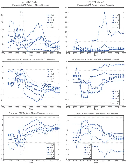
Figure 2shows fluctuation rationality results for the Min-cer and Zarnowitz (1969) regressions for the following cases: for testingH0:α=0 andβ =1 jointly for each horizon (first
row); for testingH0:α=0 (second row); and for testingH0: β=1 (third row). The figure also plots 95% confidence bands. The former is a one-sided test, whereas the latter are two-sided
t-tests. Specifically, the Mincer and Zarnowitz’s regression is Wt,m=(#θt−θ0)′V#θ,t−1(#θt−θ0) fort =m/2, . . . , P−m/2+1
and θ0=[0,1]′ (first row); the fluctuation rationality test
on the constant is Wt,mα =#α′ t V#
−1/2
α,t (second row) and that on the slope is Wt,mβ =(β#t−1) V#
−1/2
β,t (third row), where
#
Vα,t and Vβ,t# are the diagonal elements of Vθ,t# . The figure
shows that forecast rationality is rejected for horizons 0, 2, and 5 for the GDP deflator, and for horizon 1 for the GDP growth.
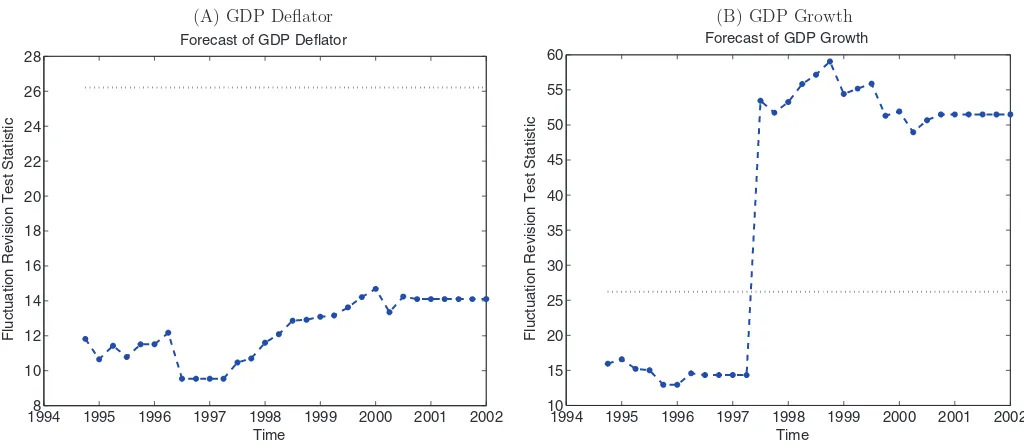
The framework discussed above can also be generalized to develop a version of the Patton and Timmermann’s (2010) optimal revision regression test (implemented with a proxy) robust to instability. We refer to this test as the “fluctuation revision” test. The fluctuation revision test is defined as in Equation (4), whereWt,m is defined by Equation (3),vt=yt, gt−h=[1, yt|t−hH, dt|h1,h2, . . . , dt|hH−1,hH], H is the maximum
forecast horizon, dt|hH−1,hH denotes the forecast revision
be-tween horizonshH−1andhH, andθ0=[0,1, . . . ,1]′.Figure 3
shows the test statistic,Wt,m, over time; the dotted lines report
the 5% critical value. According to the figures, the implications of forecast rationality considered by Patton and Timmermann (2010) are not rejected for the GDP deflator, whereas they are rejected for GDP growth (mainly in the late 1990s).
(A)GDP Deflator (B)GDP Growth
1994 1995 1996 1997 1998 1999 2000 2001 2002
0
Forecast of GDP Deflator : Mincer-Zarnowitz
h=0
1994 1995 1996 1997 1998 1999 2000 2001 2002
0
Forecast of GDP Growth : Mincer-Zarnowitz
h=0
1994 1995 1996 1997 1998 1999 2000 2001 2002
-4
Forecast of GDP Deflator : Mincer-Zarnowitz on constant
h=0
1994 1995 1996 1997 1998 1999 2000 2001 2002 -3
Forecast of GDP Growth : Mincer-Zarnowitz on constant
h=0
1994 1995 1996 1997 1998 1999 2000 2001 2002
-6
Forecast of GDP Deflator : Mincer-Zarnowitz on slope
h=0
1994 1995 1996 1997 1998 1999 2000 2001 2002
-6
Forecast of GDP Growth : Mincer-Zarnowitz on slope
h=0
Figure 2. Fluctuation rationality tests for the Mincer and Zarnowitz (1969) regressions for the following cases: for testingH0:α=0 and
β=1 jointly for each horizon (first row); for testingH0:α=0 (second row); and for testingH0:β=1 (third row). In particular, the figure
reports Equation (3) together with 95% confidence bands (dotted lines). (Color figure available online.)
(A) GDP Deflator (B) GDP Growth
19948 1995 1996 1997 1998 1999 2000 2001 2002
10 12 14 16 18
20 22 24 26 28
Forecast of GDP Deflator
Fl
u
ct
u
ation Re
v
ision Test Statistic
Time
1994 1995 1996 1997 1998 1999 2000 2001 2002
10 15 20 25 30 35 40 45 50 55 60
Forecast of GDP Growth
Fl
u
ct
u
ation Re
v
ision Test Statistic
Time
Figure 3. Fluctuation revision test over time (line with stars) for GDP deflator data (left-hand side panel) and GDP growth (right-hand side panel), together with the critical value (dotted line). (Color figure available online.)
To conclude, we found empirical evidence in favor of insta-bilities in the parameters of forecasting rationality regressions. Studying such instabilities might provide useful information as to when rejections of forecast rationality occurred, as well as their possible economic causes.
ACKNOWLEDGMENTS
The author is grateful to A. Patton and J. Wright for shar-ing their codes and data, and to K. Hirano and J. Wright for organizing the special JBES session at the American Economic Association (AEA).
[Received March 2011. Accepted August 2011.]
REFERENCES
Diebold, F. X. (2001),Elements of Forecasting(2nd ed.), Cincinnati, OH: South-Western College Publishing. [25]
Faust, J., and Wright, J. (2009), “Comparing Greenbook and Reduced Form Forecasts using a Large Realtime Dataset,” Journal of Business and Eco-nomic Statistics, 27, 468–479. [26]
Giacomini, R., and Rossi, B. (2010), “Forecast Comparisons in Unstable Envi-ronments,”Journal of Applied Econometrics, 25, 595–620. [27]
Mincer, J., and Zarnowitz, V. (1969), “The Evaluation of Economic Forecasts,” in Economic Forecasts and Expectations, ed. J. A. Min-cer, New York: National Bureau of Economic Research, pp. 81– 111. [26]
Newey, W., and West, K. (1987), “A Simple, Positive Semi-Definite, Het-eroskedasticity and Autocorrelation Consistent Covariance Matrix,” Econo-metrica, 55, 703–708. [26]
Patton, A., and Timmermann, A. (2007), “Properties of Optimal Forecasts Under Asymmetric Loss and Nonlinearity,”Journal of Econometrics, 140, 884–918. [25]
Patton, A., and Timmermann, A. (2012), “Forecast Rationality Tests Based on Multi-Horizon Bounds,”Journal of Business and Economic Statistics, forthcoming. [25]
Rossi, B. (2005), “Optimal Tests for Nested Model Selection with Un-derlying Parameter Instabilities,” Econometric Theory, 21, 962– 990. [26]
Rossi, B. (2011), “Forecasting in Unstable Environments,” inHandbook of Forecasting, Vol. 2, eds. G. Elliott and A. Timmermann, North Holland: Elsevier. Forthcoming. [25]
Rossi, B., and Sekhposyan, T. (2010), “Have Models’ Forecasting Performance Changed Over Time, and When?,” International Journal of Forecasting, 26, 808–835. [25]
Rossi, B., and Sekhposyan, T. (2011), “Forecast Optimality Tests in the Pres-ence of Instabilities,” Mimeo, Duke University. [25]