getdocdae4. 196KB Jun 04 2011 12:05:03 AM

El e c t ro n ic

Jo ur

n a l o

f P

r o

b a b i_{l i t y}

Vol. 13 (2008), Paper no. 66, pages 2014–2030. Journal URL

http://www.math.washington.edu/~ejpecp/

On the birth-and-assassination process, with an

application to scotching a rumor in a network

Abstract

We give new formulas on the total number of born particles in the stable birth-and-assassination process, and prove that it has a heavy-tailed distribution. We also establish that this process is a scaling limit of a process of rumor scotching in a network, and is related to a predator-prey dynamics.

Key words:branching process, heavy tail phenomena, SIR epidemics. AMS 2000 Subject Classification:Primary 60J80.

1

Introduction

Birth-and-assassination process

The birth-and-assassination process was introduced by Aldous and Krebs [2], it is a variant of the branching process. The original motivation of the authors was then to analyze a scaling limit of a queueing process with blocking which appeared in database processing, see Tsitsiklis, Papadimitriou and Humblet[14]. In this paper, we show that the birth-and-assassination process exhibits some heavy-tailed distribution. For general references on heavy-tail distribution in queueing processes, see for example Mitzenmacher[9]or Resnick[12]. In this paper, we will not discuss this application. Instead, we will show that the birth-and-assassination process is also the scaling limit of a rumor spreading model which is motivated by network epidemics and dynamic data dissemination (see for example,[10],[4],[11]).

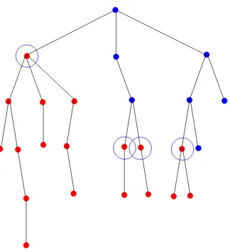
Figure 1: Illustration of the birth-and-assassination process, living particles are in red, dead particles in blue, particles at risk are encircled.

We now reproduce the formal definition of the birth-and-assassination process from[2]. LetNf =

∪∞k=0N

k_{be the set of finite k-tuples of positive integers (withN}0₌

;). Let_{Φ_n},n_∈Nf_{, be a family} of independent Poisson processes with common arrival rate λ. Let _{K_n},n_∈ Nf_{, be a family of} independent, identically distributed (iid), strictly positive random variables. Suppose the families {Φ_n}and_{K_n}are independent. The particle system starts at time 0 with only the ancestor particle, indexed by _;. This particle produces offspring at the arrival times of Φ_;, which enter the system with indices (1), (2), _{· · ·} according to their birth order. Each new particle nentering the system immediately begins producing offspring at the arrival times of{Φ_n}, the offspring ofnare indexed

(n, 1),(n, 2),_{· · ·} also according to birth order. The ancestor particle isat riskat time 0. It continues to produce offspring until time D_; = K_;, when it dies. Let k > 0 and let n= (n1,· · ·,nk−1,nk),

n′ = (n1, ...,nk−1). When a particlen′ dies (at time Dn′), nthen becomes at risk; it continues to

produce offspring until timeD_n=D_n′+K_n, when it dies. We will say that the birth-and-assassination

Theorem 1 (Aldous and Krebs). Consider a birth-and-assassination process with offspring rate λ

whose killing distribution has moment generating functionφ. Supposeφis finite in some neighborhood of 0. Ifmin_u>0λu−1φ(u)<1then the process is stable. Ifminu>0λu−1φ(u)>1then the process is

unstable.

The birth-and-assassination process is a variant the classical branching process. Indeed, if instead the particlenis at risk not when its parent dies but when the particlenwas born, then we obtain a well-studied type of branching process, refer to Athreya and Ney[5]. The populations in successive generations behave as the simple Galton-Walton branching process with mean offspring equal to

λEK_;, and so the process is stable if this mean is less than 1. The birth-and-assassination process is a variation in which the ’clock’ which counts down the time until a particle’s death does not start ticking until the particle’s parent dies.

In this paper, we will pay attention to the special case where the killing distribution is an exponen-tial distribution with intensityµ. By a straightforward scaling argument, a birth-and-assassination process with intensities(λ,µ)and a birth-and-assassination process with intensities(λµ−1_{, 1)where}

the time is accelerated by a factorµhave the same distribution. Therefore, without loss of general-ity, from now on, we will consider_B, a birth-and-assassination process with intensities(λ, 1). As a corollary of Theorem 1, we get

Corollary 1(Aldous and Krebs). If0< λ <1/4, the processB is stable. Ifλ >1/4, the processB is unstable.

In the first part of this paper, we study the behavior of the processB in the stable regime, especially asλget close to 1/4. We introduce a family of probability measures_{Pλ},λ >0, on our underlying

probability space such that under P_λ, _B is a birth-and-assassination process with intensities(λ, 1). Let λ∈(0, 1/4), we define N as the total number of born particles in B (including the ancestor particle) and

γ(λ) =sup

u_≥0 : E_λNu<∞ .

In particular, if 0< γ(λ)<∞, from Markov Inequality, for all 0< ε < γ(λ), there exists a constant

C _≥1 such that for allt_≥1,

Pλ(N>t)≤C t−γ(λ)+ε.

The numberγmay thus be interpreted as a power tail exponent. There is a simple expression forγ.

Theorem 2. For allλ∈(0, 1/4),

γ(λ) =1+

p 1−4λ

1−p1−4λ.

This result contrasts with the behavior of the classical branching process, where for all λ < 1: there exists a constant c>0 such that Eλexp(cN)<∞. This heavy tail behavior of the

birth-and-assassination process is thus a striking feature of this process. Near criticality, asλ ↑1/4, we get

γ(λ)_∼1, whereas asλ↓0, we findγ(λ)_∼(2λ)−1. By recursion, we will also compute the moments ofN.

Theorem 3. (i) For all p≥2,EλNp<∞if and only ifλ∈(0,p(p+1)−2).

(ii) Ifλ∈(0, 1/4],

E_λN= 2

(iii) Ifλ∈(0, 2/9),

E_λN2= 2

3p1₋4λ−1. (2)

Theorem 3(i) is consistent with Theorem 2: λ ∈ (0,p(p+1)−2_{) is equivalent to p ∈ [1,(1+}

p

1₋4λ)(1₋p1₋4λ)−1) . Theorem 3(ii) implies a surprising discontinuity of the function

λ 7→E_λN at the critical intensity λ = 1/4: lim_λ↑1/4E_λN = 2. Again, this discontinuity contrasts with what happens in a standard Galton-Watson process near criticality, where for 0 < λ < 1, E_λN= (1₋λ)−1. We will prove also that this discontinuity is specific toλ=1/4 and for allp_≥2, lim_λ↑p(p+1)−2E_λ[Np] =∞. We will explain a method to compute all integers moments ofN by

re-cursion. The third moment has already a complicated expression (see §2.5.1). From Theorem 3(ii), we may fill the gap in Corollary 1.

Corollary 2. Ifλ=1/4, the process_B is stable.

In Section 2, we will prove Theorems 2 and 3 by exhibiting a Recursive Distributional Equation (RDE) for a random variable related toN. Unfortunately, our method does not give much insights on the heavy-tail phenomena involved in the birth-and-assassination process.

Rumor scotching process

We now define the rumor scotching process on a graph. It is a nonstandard SIR dynamics (see for example [10] or [4] for some background). This process represents the dynamics of a ru-mor/epidemic spreading on the vertices of a graph along its edges. A vertex may be unaware of the rumor/susceptible (S), aware of the rumor and spreading it as true/infected (I), or aware of the rumor and trying to scotch it/recovered (R).

More formally, we fix a connected graph G = (V,E), and let _PV denote the set of subsets of V

and_X = (_{PV × {}S,I,R_})V. The spread of the rumor is described by a Markov process on _X. For

X = (Xv)v∈V∈ X, withXv= (Av,sv),Av is interpreted as the set of neighbors ofvwhich can change the opinion ofv on the veracity of the rumor. If(uv)_∈E, we define the operationsE_uv andE_v on X by(X+E_uv)_w= (X₋E_v)_w =X_w, ifw₆=vand(X+E_uv)_v = (A_{v∪ {}u_},I),(X₋E_v)_v= (_;,R). Let

λ >0 be a fixed intensity, the rumor scotching process is the Markov process with generator:

K(X,X+E_uv) = λ1(s_u=I)1((u,v)_∈E)1(s_v6=R),

K(X,X₋E_v) = 1(s_v=I)X

u∈Av

1(s_u=R),

and all other transitions have rate 0. Typically, at time 0, there is non-empty finite set of I-vertices and there is a vertexvsuch thatAv contains aR-vertex. The absorbing states of this process are the states withoutI-vertices. The case when at time 0,A_v is the set to all neighbors ofvis interesting in its own (there,A_v does not evolve befores_v=R).

variant of the two-species Richardson model with prey and predators, see for example Häggström and Pemantle[6], Kordzakhia and Lalley[8]. Nothing is apparently known on this process.

In Section 3, we show that the birth-and-assassination process is the scaling limit, asngoes to infin-ity, of the rumor scotching process whenGis the complete graph overnvertices and the intensity is

λ/n(Theorem 4).

2

Integral equations for the birth-and-assassination process

2.1

Proof of Theorem 3 for the first moment

In this paragraph, we prove Theorem 3(ii). LetX(t)_∈[0,+_∞]be the total number of born particles in the processB given that the root cannot die before timet, andY(t)be the total number of born particles given that the root dies at timet. By definition, ifDis an exponential variable with mean 1 independent ofY, thenN=d X(0)=d Y(D), where the symbol=d stands for distributional equality. We notice also that the memoryless property of the exponential variable implies X(t)=d Y(t+D). The recursive structure of the birth-and-assassination process leads to the following equality in distribution

Y(t)=d 1+ X

i:ξi≤t

X_i(t−ξ_i)=d 1+ X

i:ξi≤t

X_i(ξ_i),

whereΦ =_{ξi}i∈N is a Poisson point process of intensityλand(Xi),i∈N, are independent copies ofX. Note that since all variables are non-negative, there is no issue with the caseY(t) = +_∞. We obtain the following RDE for the random functionY:

Y(t)=d 1+ X

i:ξi≤t

Y_i(ξi+Di), (3)

where Y_i, andD_i are independent copies ofY andDrespectively. This last RDE is the cornerstone of this work.

Assuming that EλN<∞we first prove that necessarilyλ∈(0, 1/4). For convenience, we often drop

the parameterλ in Eλ and other objects depending onλ. From Fubini’s theorem, EX(0) =EN = R∞

0 EY(t)e

−t_{d tand therefore EY(t)<}

∞for almost allt_≥0. Note however that sincet _7→Y(t)is monotone for the stochastic domination, it implies that EY(t)<∞for allt>0. The same argument gives the next lemma.

Lemma 1. Let t>0and u>0, ifE[Nu]<∞thenE[Y(t)u_]<∞.

Now, taking expectation in (3), we get

EY(t) = 1+λ

Z t

0

Z ∞

0

EY(x+s)e−sdsd x.

Let f₁(t) =EY(t), it satisfies the integral equation, for allt_≥0,

f₁(t) =1+λ

Z t

0

ex

Z ∞

x

Taking the derivative once and multiplying bye−t, we get: f₁′(t)e−t=λR_t∞f₁(s)e−sds. Then, taking the derivative a second time and multiplying byet: f₁′′(t)₋f₁′(t) =₋λf₁(t). So, finally, f₁ solves a linear ordinary differential equation of the second order

x′′₋x′+λx=0, (5) with initial conditionx(0) =1. Ifλ >1/4 the solutions of (5) are

x(t) =et/2(cos(t

p

4λ−1) +asin(t

p

4λ−1)),

for some constant a. Since f₁(t)is necessarily positive, this leads to a contradiction and EN =_∞. Assume now that 0< λ <1/4 and let

∆ =p1₋4λ , α= 1−∆

2 and β=

1+ ∆

2 . (6)

(α,β)are the roots of the polynomialX2₋X+λ=0. The solutions of (5) are

x_a(t) = (1−a)eαt+aeβt

for some constanta. Whereas, forλ=1/4,α=1/2 and the solutions of (5) are

xa(t) = (at+1)et/2.

For 0< λ≤1/4, we check easily that the functions x_awitha_≥0 are the nonnegative solutions of the integral equation (4).

It remains to prove that if 0 < λ ≤ 1/4 then EN < ∞ and f1(t) = eαt. Indeed, then EN =

R∞

0 f1(t)e

−t_{d t= (1−α)}−1 _{as stated in Theorem 3(ii). To this end, define f}(n)

1 (t) =E min(Y(t),n),

from (3),

min(Y(t),n)_≤st1+ X

i:ξi≤t

min(Y_i(ξi+Di),n).

Taking expectation, we obtain, for allt_≥0,

f₁(n)(t)_≤1+λ

Z t

0

ex

Z ∞

x

f₁(n)(s)e−sdsd x. (7)

We now state a lemma which will be used multiple times in this paper. We define

γ(λ) = (1+ ∆)/(1₋∆) =β/α. (8)

Let 1 < u < γ (or equivalently λ < u(u+1)−2), we define_Hu, the set of measurable functions

h:[0,∞)_→[0,∞)such thathis non-decreasing and sup_t≥0h(t)e−uαt <∞. LetC >0, we define the mapping from_Huto_Hu,

Ψ:h_7→C euαt+λ

Z t

0

ex

Z ∞

x

h(s)e−sdsd x.

In order to check thatΨis indeed a mapping from_Huto_Hu, we use the fact that if 1<u< γ, then

uα <1. Note also that if 1<u< γ, thenuα−λ−u2α2_{>0. Ifλ=1/4, we also define the mapping}

from_H1 to_H1,

Φ:h_7→1+1

4

Z t

0

ex

Z ∞

x

h(s)e−sdsd x.

Lemma 2. (i) Let1<u< γand f _{∈ Hu}such that f _≤Ψ(f). Then for all t_≥0,

f(t)_≤C uα(1−uα) uα−λ−u2_α2e

uαt

−C λ

uα−λ−u2_α2e

αt_.

(ii) Ifλ=1/4and f ∈ H1 is such that f ≤Φ(f), then for all t≥0,

f(t)_≤et/2.

Before proving Lemma 2, we conclude the proof of Theorem 3(ii). For 0< λ <1/4, from (7), we may apply Lemma 2(i) applied to 1<u< β/α,C=1. We get that

f₁(n)(t)_≤C_ueαut

for some Cu > 0. The monotone convergence theorem implies that f1(t) =limn→∞f

(n)

1 (t) exists

and is bounded byC_ueαut. Therefore f1 solves the integral equation (4) and is equal to xa for some

a _≥0. From what precedes, we get x_a(t)_≤C_ueαut, however, sinceαu< β, the only possibility is

a=0 and f1(t) =eαt.

Similarly, ifλ=1/4, from Lemma 2(ii), f₁(t)_≤et/2. This proves that f₁ is finite, and we thus have

f1=xa for somea≥0. Again, the only possibility isa=0 since xa(t)≤et/2 impliesa=0.

Proof of Lemma 2.(i). The fixed points of the mappingΨare the functionsh_a,bsuch that

h_a,b(t) =aeαt+beβt+C uα(1−uα) uα−λ−u2_α2e

uαt_,

witha+b+C_uu_αα(1−uα)

−λ−u2_α2 =C. The only fixed point inHuish_∗:=ha_∗,0witha∗=−Cλ/(uα−λ−u2α2).

Let_Cu denote the set of continuous functions in_Hu, note thatΨis also a mapping from_Cu to_Cu. Now let g0∈ Cu and fork≥1, gk= Ψ(gk−1). We first prove that for all t≥0 , limkgk(t) =h∗(t).

If 1<u< γthenuα(1₋uα)> λand _uu_αα(1−uα)

−λ−u2_α2 is positive. We deduce easily that if g0(t)≤ Leuαt

theng1(t) = Ψ(g)(t)≤C euαt+_uα(1L₋λ_uα)(euαt−1)≤L1euαt, with L1= (C+_uα(1L₋λ_uα)). By recursion,

we obtain that lim sup_kgk(t) ≤ L∞euαt, with L∞ = Cuα(1−uα)/(uα−λ−u2α2) < ∞. From

Arzela-Ascoli’s theorem,(g_k)_k∈N is relatively compact inCu and any accumulation point converges toh_∗(sinceh_∗is the only fixed point ofΨin_Cu).

Now since f _{∈ Hu}, there exists a constant L>0 such that for allt _≥0, f(t)_≤g₀(t):= Leuαt. The monotonicity of the mappingΨimplies thatΨ(f)_≤Ψ(g₀) =g₁. By assumption, f _≤Ψ(f)thus by recursion f ≤limngn=h∗.

(ii). The functionx₀(t) =et/2 is the only fixed point ofΦin_H1. Moreover, ifg(t)_≤C et/2then we also haveΦ(g)(t)_≤C et/2. Then, if gis continuous, arguing as above, from Arzela-Ascoli’s theorem,

(Φk(g))_k∈N converges to x0. We conclude as in (i). ƒ

2.2

Proof of Theorem 3(i)

We define f_p(t) = Eλ[Y(t)p]. As above, we often drop the parameterλ in Eλ and other objects

depending onλ.

(i) Ifλ∈(0,p(p+1)−2), then f_p(t) =Q_p(eαt).

(ii) Ifλ≥p(p+1)−2_{, then f}

p(t) =∞,

Note that if such polynomialQpexists thenQp(x)≥1 for allx≥1. Note also thatλ∈(0,p(p+1)−2) implies that p < γ= β/α (whereγwas defined by (8)), and thus pα < β <1. Hence Lemma 3 implies Theorem 3(i) since E[Np] =R f_p(t)e−td t.

Letκp(X) denote the pthcumulant of a random variable X whose moment generating function is defined in a neighborhood of 0: ln EeθX =P_p≥0κp(X)θp/p!. In particularκ0(X) =0,κ1(X) =EX

andκ2(X) =VarX. Using the exponential formula

E expX

ξi∈Φ

h(ξi,Zi) =exp(λ

Z ∞

0

(Eeh(x,Z)₋1)d x), (9)

valid for all non-negative function hand iid variables (Zi),i ∈N, independent of Φ = {ξi}i∈N a Poisson point process of intensityλ, we obtain that for all p≥1,

κp



 

X

i:ξi≤t

h(ξi,Zi)





=λ

Z t

0

Ehp(x,Z)d x. (10)

Due to this last formula, it will be easier to deal with the cumulantg_p(t) =κp(Y(t)). By recursion, we will prove the next lemma which implies Lemma 3.

Lemma 4. Let p≥2, there exists a polynomial Rp with degree p, positive on[1,∞)such that, for all

t>0,

(i) Ifλ∈(0,p(p+1)−2_{), then f}

p(t)<∞and gp(t) =Rp(eαt).

(ii) Ifλ≥p(p+1)−2, then f_p(t) =_∞,

Proof of Lemma 4. In §2.1, we have computed f_p for p= 1 and foundR₁(x) = x. Let p _≥2 and assume now that the statement of the Lemma 4 holds forq = 1,_{· · ·},p−1. We assume first that

f_p(t)<∞, we shall prove that necessarilyλ∈(0,p(p+1)−2_)andg

p(t) =Rp(eαt). Without loss of generality we assume that 0< λ <1/4. From Fubini’s theorem, using the linearity of cumulants in (3) and (10), we get

g_p(t) = λ

Z t

0

Z ∞

0

E[Y(x+s)p]e−sdsd x

= λ

Z t

0

ex

Z ∞

x

fp(s)e−sdsd x, (11)

(note that Fubini’s Theorem implies the existence of fp(s) for all s > 0). From Jensen inequality

fp(t)≥ g1(t)p=epαt and the integral

R∞

x e

pαs_e−s_{dsd x is finite if and only ifpα <1. We may thus} assume thatpα <1. We now recall the identity: EXp=P_πQ_I∈πκ_|I|(X), where the sum is over all

Σ_p−1(x₁,_{· · ·},x_p−1)is a polynomial inp₋1 variables with non-negative coefficients and each of its

(recall that pα < 1). Now we take the derivative of this last expression, multiply by e−t and take the derivative again. We get thatg_pis a solution of the differential equation:

x′′₋x′+λx=₋ with Equation (11) which asserts thatgp(t)is positive.

for some constantC>0. We take the expectation in (14) and use Slyvniak’s theorem to obtain

So finally for a suitable choice ofC,

|f_p(n)(t)_≤C epαt+λ

Since f₁(t) =eαt andα2=α−λ, g₂ satisfies the integral equation:

We deduce that g2solves an ordinary differential equation:

x′′−x′+λx =₋λe2αt,

2, we shall prove two statements

If E[Nu]<∞thenu_≤γ, (17)

to deduce that there exists 0< ε < λsuch that

Let ˜λ=λ−ε, ˜α=α(λ˜), ˜β=β(λ˜), we may assume thatεis small enough to ensure also that

uα >β˜. (21)

(Indeed, for allλ∈(0, 1/4),α(λ)γ(λ) =β(λ)and the mappingλ7→β(λ)is obviously continuous). We compute a lower bound from (19) as follows:

f_u(t) _≥ 1+λ˜

The statement (18) is a direct consequence of Lemmas 2 and 5. Indeed, note that f_u(n)≤nu, thus by Lemma 2, for all t≥0, f_u(n)(t)_≤C1euαt for some positive constant C1independent of n. From the

Monotone Convergence Theorem, we deduce that, for allt ≥0, f_u(t)_≤C1euαt. It remains to prove

Lemma 5.

(which follows from the inequality(Py_i)v _≤Py_iv). Then from (3) we get the stochastic

domina-2.5

Some comments on the birth-and-assassination process

2.5.1 Computation of higher moments

It is probably hard to derive an expression for all moments ofN, even if in the proof of Lemma 4, we have built an expression of the cumulants ofY(t) by recursion. However, exact formulas become quickly very complicated. The third moment, computed by hand, gives

f₃(t) =3 3λ−α

2.5.2 Integral equation of the Laplace transform

It is also possible to derive an integral equation for the Laplace transform of Y(t): L_θ(t) =

Taking twice the derivative, we deduce that, for allθ >0,Lθ solves the differential equation:

x′′x−x′2−x′x+λx2(x−1) =0.

2.5.3 Probability of extinction

Ifλ >1/4 from Corollary 1, the probability of extinction ofB is strictly less than 1. It would be very interesting to have an asymptotic formula for this probability asλget close to 1/4 and compare it with the Galton-Watson process. To this end, we defineπ(t)as the probability of extinction of_B given than the root cannot die beforet. With the notation of Equation (3),π(t)satisfies

π(t) =E Y i:ξi≤t+D

π(t+D−ξi) =E

Y

i:ξi≤t+D

π(ξi),

Using the exponential formula (9), we find that the functionπsolves the integral equation:

π(t) =et

Z ∞

t exp

‚

−(λ+1)s+λ

Z s

o

π(x)d x

Œ

ds.

After a quick calculation, we deduce that πis solution of the second order non-linear differential equation

x′−x′′

x−x′ =λ(x−1).

Unfortunately, we have not been able to get any result on the functionπ(t) from this differential equation.

3

Rumor scotching in a complete network

3.1

Definition and result

0 1

Figure 2: The graphG₆.

We consider the rumor scotching process on the graphGn on{0,· · ·,n}obtained by adding on the complete graph on{1,· · ·,n}the edge(0, 1), see Figure 2. LetPnbe the set of subsets of{0,· · ·,n}. With the notation in introduction, the rumor scotching process on G_n is the Markov process on Xn= (_{Pn× {}S,I,R})nwith generator, forX = (Ai,si)0≤i≤n,

K(X,X+Ei j) =λn−11(si=I)1(sj6=R),

K(X,X₋E_j) =1(s_j=I)

n

X

i=1

1(i_∈A_j)

!

and all other transitions have rate 0. At time 0, the initial state isX(0) = (X_i(0))_0≤i≤nwithX₀(0) = (_;,R),X1(0) = ({0},I)and fori≥2,Xi(0) = (;,S).

With this initial condition, the process describes the propagation of a rumor started from vertex 1 at time 0. After an exponential time, vertex 1 learns that the rumor is false and starts to scotch the rumor to the vertices it had previously informed. This process is a Markov process on a finite set with as absorbing states, all states withoutI-vertices. We defineN_nas the total number of recovered vertices in_{1, . . . ,n_}when the process stops evolving. We also define Y_n(t)as the distribution N_n

given that vertex 1 is recovered at timet. We have the following

Theorem 4. (i) If 0 < λ ≤ 1/4 and t ≥ 0, as n goes to infinity, N_n and Y_n(t) converge weakly respectively to N and Y(t)in the birth-and-assassination process of intensityλ.

(ii) Ifλ >1/4, there existsδ >0such that

lim inf

n Pλ(Nn≥δn)>0.

The proof of Theorem 4 relies on the convergence of the rumor scotching process to the birth-and-assassination process, exactly as the classical SIR dynamics converges to a branching process as the size of the population goes to infinity.

3.2

Proof of Theorem 4

3.2.1 Proof of Theorem 4(i)

The proof of Theorem 4 relies on an explicit contruction of the rumor scotching process. Let

(ξ(n)_{i j} ), 1 _≤ i < j _≤ n, be a collection of independent exponential variables with parameter λn−1

and, for all 1 _≤ i _≤ j, let D_{i j} be an independent exponential variable with parameter 1. We set

D_ji = D_{i j} andξ(n)_ji = ξ(n)_{i j} . A network being a graph with marks attached on edges, we define Kn as the network on the complete graph of_{1,_{· · ·},n_}where the mark attached on the edge(i j)is the pair(ξ(n)_{i j} ,D_{i j}). Now, the rumor scotching process is built on the network_Kn by settingξ(n)_{i j} as the time for the infected particleito infect the particle j andDi j as the time for the recovered particlei to recover the particle jthat it had previously infected.

The network_Knhas a local weak limit asngoes to infinity (see Aldous and Steele[3]for a definition of the local weak convergence). This limit network ofKn isK, the Poisson weighted infinite tree (PWIT) which is described as follows. The root vertex, say _;, has an infinite number of children indexed by integers. The marks associated to the edges from the root to the children are(ξi,Di)i≥1

where{ξi}i≥1is the realization of a Poisson process of intensityλonR+ and(Di)i≥1 is a sequence

of independent exponential variables with parameter 1. Now recursively, for each vertex i_≥1 we associate an infinite number of children denoted by(i, 1),(i, 2),_{· · ·} and the marks on the edges from

i to its children are obtained from the realization of an independent Poisson process of intensityλ

on R_{+ and a sequence of independent exponential variables with parameter 1. This procedure is} continued for all generations. Theorem 4.1 in[3]implies the local weak convergence of_Kn to_K (for a proof see Section 3 in Aldous[1]).

Fors>0 andℓ∈N_{, letKn[s,ℓ]be the network spanned by the set of vertices j ∈ {1,· · ·,n}such} that there exists a sequence(i₁,_{· · ·},i_k) with i₁ = 1, i_k = j, k _≤ ℓ and max(ξ(n)_i

1i2,· · ·,ξ

(n)

ik−1ik) ≤ s.

If τn is the time elapsed before an absorbing state is reached, we get that 1(τn ≤ s)1(Nn ≤ ℓ)is measurable with respect toKn[s,ℓ]. From Theorem 4.1 in[3], we deduce that1(τn≤s)1(Nn≤ℓ) converges in distribution to1(τ≤ s)1(N _≤ ℓ) where τis the time elapsed before all particles die in the birth-and-assassination process. If 0< λ <1/4,τis almost surely finite and we deduce the statement (i).

3.2.2 Proof of Theorem 4(ii)

In order to prove part (ii) we couple the birth-and-assassination process and the rumor scotching process. We use the above notation and build the rumor scotching process on the networkKn. If

X = ((A_i,s_i)_0≤i≤n)_{∈ Xn}, we defineI(X) =_{1_≤i_≤n:s_i =I_}andS(X) =_{1_≤i_≤n:s_i=S_}. Let X = X_n(u) _{∈ Xn} be the state of the rumor scotching process at time u_≥ 0. Let i _∈ I(X), we reorder the variables (ξ(n)_{i j} )_j∈S(X) in non-decreasing order: ξ(n)_{i j}

1 ≤ · · · ≤ ξ

(n)

i j_|S(X)|. Define ξ

(n) i j0 = 0,

from the memoryless property of the exponential variable, for 1 ≤ k ≤ |S(X)_|, ξ(n)_{i j}

k −ξ

(n) i jk−1 is an

exponential variable with parameter λ(_|S(X)_{| −}k+1)/n independent of (ξ(n)_{i j}

ℓ −ξ

(n)

i jℓ−1, ℓ < k).

Therefore, for all 1≤k≤ |S(X)_|, the vector(ξ(n)_{i j} 1,· · ·,ξ

(n)

i jk)is stochastically dominated

component-wise by the vector(ξ1,· · ·,ξk)where{ξj}j≥1 is a Poisson process of intensity λ(|S(X)| −k+1)/n

on R_{+ (i.e. for all 0 ≤ t1 ≤ · · · ≤ tk, P(ξ}(n)

i j1 ≥ t1,· · ·,ξ

(n)

i jk ≥ tk) ≤ P(ξ1 ≥ t1,· · ·,ξk ≥ tk)). In

particular if_|S(X)_{| ≥}(1₋δ)n, with 0< δ <1/2, then(ξ(n)_i1 ,_{· · ·},ξ(n)_i⌊nδ⌋)is stochastically dominated component-wise by the first_⌊nδ⌋arrival times of a Poisson process of intensityλ(1₋2δ).

Now, letδ >0 such thatλ′=λ(1₋2δ)>1/4. We define S_u(n),I_u(n),R(n)_u , as the number ofS,I,R -particles at timeu≥0 in_Kn, and I_u′ as the number of particles "at risk" at timeuin the birth-and-assassination process with intensityλ′. Letτn=inf{u≥0 :Su(n)≤(1−δ)n}. Note that if 0≤u≤τn then anyI-particle has infected less than⌊δn⌋S-particles. From what precedes, we get

S_u(n)1(u≤τn)≤st n−Iu′.

So thatS(n)_{u ≤st}max(n₋I_u′,(1₋δ)n). In particular, sinceN_n≥sup_u≥0(n₋S(n)_u ), we get

Pλ(Nn≥δn)≥Pλ′(lim sup

u→∞

I_u′ =_∞).

Finally, it is proved in[2]that ifλ′>1/4 then P_λ′(lim sup_u→∞I_u′ =∞)>0.

Acknowledgement

References

[1] D. Aldous. Asymptotics in the random assignment problem. Probab. Theory Related Fields, 93(4):507–534, 1992. MR1183889

[2] D. Aldous and W. Krebs. The “birth-and-assassination” process. Statist. Probab. Lett., 10(5):427–430, 1990. MR1078244

[3] D. Aldous and M. Steele. The objective method: probabilistic combinatorial optimization and local weak convergence. 110:1–72, 2004. MR2023650

[4] H. Andersson. Epidemic models and social networks. Math. Sci., 24(2):128–147, 1999. MR1746332

[5] K. Athreya and P. Ney. Branching processes. Springer-Verlag, New York, 1972. MR0373040

[6] O. Häggström and R. Pemantle. First passage percolation and a model for competing spatial growth. J. Appl. Probab., 35(3):683–692, 1998. MR1659548

[7] G. Kordzakhia. The escape model on a homogeneous tree. Electron. Comm. Probab., 10:113– 124 (electronic), 2005. MR2150700

[8] G. Kordzakhia and S. P. Lalley. A two-species competition model on Zd_{. Stochastic Process.}

Appl., 115(5):781–796, 2005. MR2132598

[9] M. Mitzenmacher. A brief history of generative models for power law and lognormal distribu-tions. Internet Math., 1(2):226–251, 2004. MR2077227

[10] M. Newman, A.-L. Barabási, and D. J. Watts, editors. The structure and dynamics of networks. Princeton Studies in Complexity. Princeton University Press, Princeton, NJ, 2006. MR2352222

[11] K. Ramamritham and P. E. Shenoy. Special issue on dynamic information dissemination. IEEE Internet Computing, 11:14–44, 2007.

[12] S. I. Resnick. Heavy-tail phenomena. Springer Series in Operations Research and Financial Engineering. Springer, New York, 2007. Probabilistic and statistical modeling. MR2271424

[13] D. Richardson. Random growth in a tessellation. Proc. Cambridge Philos. Soc., 74:515–528, 1973. MR0329079