Statistics authors titles recent submissions

Parameter Regimes in Partial Functional

Panel Regression

∗

_{Dominik Liebl}

University of Bonn

Institute for Financial Economics and Statistics

dliebl@uni-bonn.de

and

Fabian Walders

University of Bonn

BGSE & Institute for Financial Economics and Statistics

fwalders@uni-bonn.de

Abstract

We propose a partial functional linear regression model for panel data with time varying parameters. The parameter vector of the multivariate model component is allowed to be completely time varying while the function-valued parameter of the functional model component is assumed to change over K <_∞ unknown parameter regimes. We derive consistency for the suggested estimators and for our classifica-tion procedure used to detect the K unknown parameter regimes. In addition, we derive the convergence rates of our estimators under a double asymptotic where we differentiate among different asymptotic scenarios depending on the relative order of the panel dimensions n and T. The statistical model is motivated by our real data application, where we consider the so-called “idiosyncratic volatility puzzle” using high frequency data from the S&P500.

Keywords: functional data analysis, mixed data, partial functional linear regression model, classification, idiosyncratic volatility puzzle

∗_{We want to thank Alois Kneip (University of Bonn) and Michael Vogt (University of Bonn) for fruitful}

discussions and valuable comments which helped to improve this research work.

1

Introduction

The availability of mixed—functional and multivariate—data types and the need to analyze such data types appropriately, has trigged the development of new statistical models and procedures. In this work we consider the so-called partial functional linear model for scalar responses, which combines the classical functional linear regression model (see, e.g.,

Hall and Horowitz, 2007) with the classical multivariate regression model. This model was first proposed by Zhang et al. (2007) and Schipper et al. (2008)—two mixed effects modeling approaches. The first theoretical work is by Shin (2009), who uses a functional-principal-components-based estimation procedure and derives convergence rates for the case of independent cross-sectional data. Recently, the partial functional linear regression model was extended in several directions. Shin and Lee (2012) consider the case of prediction,Lu et al. (2014) and Tang and Cheng (2014) focus on quantile regression, Kong et al. (2016) consider the case of a high-dimensional multivariate model component, Peng et al. (2016) allow for varying coefficients in the multivariate model component, andWang et al.(2016) and Ding et al. (2017) are concerned with a functional single-index model component.

Motivated by our real data application, we deviate from this literature and contribute a new partial functional linear panel regression model with time varying parameters allowing forK <∞latent parameter regimes that can be estimated from the data. In the theoretical part of this work we show consistency of our estimators and of our unsupervised classifica-tion procedure identifying theKparameter regimes. In addition, we derive the convergence rates of our estimators under a double asymptotic where we differentiate among different asymptotic scenarios depending on the relative order of the panel dimensions n and T.

The consideration of time varying parameters is quite novel in the literature on func-tional data analysis. To the best of our knowledge, the only other work concerned with this issue is Horv´ath and Reeder(2012), who focus on testing the hypothesis of a time constant parameter function in the case of a classical fully-functional regression model. Closely re-lated to the partial functional linear model is the so-called Semi-Functional Partial Linear (SFPL) proposed by Aneiros-P´erez and Vieu(2006), where the functional component con-sists of a nonparametric functional regression model instead of a functional linear regression model. The SFPL model is further investigated by Aneiros-P´erez and Vieu (2008), Lian

(2011),Zhou and Chen(2012), andAneiros-P´erez and Vieu(2013), among others. Readers with a general interest in functional data analysis are referred to the textbooks of Ramsay and Silverman (2005), Ferraty and Vieu (2006), Horv´ath and Kokoszka (2012), and Hsing and Eubank (2015).

The usefulness of our model and the applicability of our estimation procedure is demon-strated by means of a simulation study and a real data application. For the latter we con-sider the so-called “idiosyncratic volatility puzzle” using high frequency stock-level data from the S&P500. Our model allows us to consider this puzzle at a much less aggregated time scale than considered so far in the literature. This leads to new insights into the temporal heterogeneity in the pricing of the idiosyncratic risk component.

involved. The finite sample performance of the estimators is explored in Section6. Section

7 offers an empirical study examining regime dependent pricing of idiosyncratic risk in the US stock market. Section 8 contains a short conclusion. All proofs can be found in the online supplement supporting this article.

2

Model

We introduce a partial linear regression model for panel data which allows us to model the time varying effect of a square integrable random function Xit ∈ L2([0,1]) on a scalar

response yit in the presence of a finite dimensional random variablezit ∈RP. Indexing the

cross-section units i= 1, . . . , nand time points t= 1, . . . , T, our statistical model reads as

yit =µt+

Z 1

0

αt(s)Xit(s)ds+βt⊤zit+ǫit, (1)

where µt is a time fixed effect1, αt ∈ L2([0,1]) is a time varying deterministic functional

parameter,βt∈RP is a time varying deterministic parameter vector, andǫitis a scalar error

term with finite but potentially time heteroscedastic variances (see also our assumptions in Section 4).

The unknown function-valued parameters αt are assumed to differ across unknown

time regimes Gk ⊂ {1, . . . , T}. That is, each regime Gk is associated with a regime specific

parameter function Ak ∈L2[0,1], such that

αt(s)≡Ak(s) if t∈Gk. (2)

The regimes G1, . . . , GK are mutually exclusive subsets of {1, . . . , T} and do not have to

consist of subsequent time pointst. We have in mind the situation whereGk is a collection

of time points t that belong to the kth risk regime. The kth risk regime is described by the function-valued slope parameterAk—the vector-valued slope parametersβtdescribe the

marginal effects of additional control variableszit. The joint and the marginal distributions

of Xit,zit and ǫit are allowed to vary over the different regimesGk.

Model (1) nests several different model specifications. It might be the case thatK = 1 and hence G1 = {1, . . . , T}. In this situation the effect of the random function on the response is time invariant. The classical functional or the classical multivariate linear regression model are obtained if βt= 0 or αt = 0 for allt= 1, . . . , T.

3

Estimation

Our objective is to estimate the model parameters Ak, βt, and the regimes G1, . . . , GK

from realizations of the random variables {(yit, Xit, zit) : 1 ≤ i ≤ n, 1 ≤ t ≤ T}. For

this, we propose a three-step estimation procedure. The first step is a pre-estimation step where model (1) is fitted to the data separately for each t= 1, . . . , T. This pre-estimation

1

We use the termtime fixed effect in the sense thatµtis a latent time specific random variable, which

step reveals information about the regime memberships, which is used in the second step where we apply our unsupervised classification procedure in order to estimate the regimes

G1, . . . , GK. The third step is the final estimation step, in which we improve estimation of

the functional parameter Ak by employing the information about the regime membership

gathered in step two. The general procedure is inspired by the work of Vogt and Linton

(2017), but differs from it as we consider a functional data context which demands for a different estimation procedure. In the following we explain the three estimation steps in more detail:

Step 1 In this step, we pre-estimate the parameters αt and compute the final estimates

of βt separately for each t = 1, . . . , T. Estimation starts from removing the fixed effect

µt using a classical within-transformation. For this we denote the centered variables as

yc

it = yit −y¯t, Xtic = Xit−X¯t, zcit = zit−z¯it, and ǫcit = ǫit−¯ǫit, where ¯yt = n−1Pni=1yit,

¯

Xt=n−1Pn_i=1Xit, ¯zt =n−1Pn_i=1zit, and ¯ǫt=n−1Pn_i=1ǫit. Then, the within-transformed

version of model (1) is

y_itc =

Z 1

0

αt(s)Xitc(s)ds+βt⊤zitc +ǫcit.

By adapting the methodology inHall and Horowitz(2007), we estimate the slope parameter

αtusing (t-wise) truncated series expansions ofαtandXit, i.e.,αt(s)≈P_jm₌₁t hαt,φˆjtiφˆjt(s) =

Pmt

j=1ajtφˆjt(s) and Xitc(s)≈

Pmt

j=1hXitc,φˆjtiφˆjt(s), where ˆφjt denotes the eigenfunction

cor-responding to the jth largest eigenvalue ˆλjt of the empirical covariance operator ˆΓt, with

(ˆΓtx)(u) :=

Z 1

0

ˆ

KXt(u, v)dv for all x∈L

2_([0,1])

and KˆXt(u, v) := 1

n

n

X

i=1

X_itc(u)X_itc(v).

The eigenfunctions ˆφjtand eigenvalues ˆλjtare defined as the solutions of the eigen-equations

R1

0 KˆXt(u, v) ˆφjt(u)dv = ˆλjtφˆjt(u), wherehφˆjt,φˆℓti= 1 for allj =ℓandhφˆjt,φˆℓti= 0 ifj 6=ℓ, wherej, ℓ∈ {1,2, . . . , n}. This leads to the following pre-estimators of the functional slope parameter αt and the final estimators of the vector-valued slope parameterβt:

ˆ

αt= mt

X

j=1

ˆ

ajtφˆjt, with ˆajt = ˆλ−jt1

1

n

n

X

i=1 hXc

it,φˆjti(yitc −βˆt⊤zitc), and

ˆ

βt=

h

ˆ

Kz,t−Φˆt( ˆKzX,t)

i−1h

ˆ

Kzy,t−Φˆt

ˆ

KyX,t

i

where

ˆ

K_z,t:= 1

n

n

X

i=1 zc

itzitc⊤, KˆzX,t(s) := [ ˆKz1X,t(s), . . . ,KˆzPX,t(s)]

⊤_{, Kˆ}

zy,t := [ ˆKz1y,t, . . . ,KˆzPy,t]

⊤_,

ˆ

KyX,t(s) :=

1

n

n

X

i=1

y_itcX_itc(s), KˆzpX,t(s) := 1

n

n

X

i=1

z_p,itc X_itc(s), Kˆzpy,t:= 1

n

n

X

i=1

z_p,itc y_itc,

ˆ

Φt(g) := [ ˆΦ1,t(g), . . . ,ΦˆP,t(g)]⊤, Φˆp,t(g) := mt

X

j=1

hKˆzpX,t,φˆjtihφˆjt, gi ˆ

λjt

for any g _∈L2([0,1]),

and Φˆt( ˆKzX,t) := [ ˆΦp,t( ˆKzqX,t)]1≤p≤P, 1≤q≤P;

see Shin (2009) for similar estimators in a cross-section context.

For our theoretical analysis, we let mt = mt,nT → ∞ as n, T → ∞. In practice, the

cut-off parametermtcan be chosen, for instance, by Cross Validation (CV) or by a suitable

information criterion as introduced in Section 5.

Besides computing the final estimates ˆβt of βt, this first estimation step is intended to

pave the way for the classification procedure in Step 2 where we aim to detect systematic differences in the estimates ˆαt and ˆαs across different time points t 6= s. For this it

is necessary to distinguish systematically large from small differences between estimators, which can be achieved by comparing these differences to an appropriate threshold. However, the estimators ˆαt are not well suited for deriving a practically useful threshold parameter.

We, therefore, compute the following transformed estimates, for which it is straightforward to derive a valid threshold parameter using distributional arguments (see Section 5):

ˆ

α(∆)t := m

X

j=1

ˆ

λ1_jt/2

ˆ

σǫ,t

ˆ

ajtφˆjt, (3)

where ˆσ2

ǫ,t :=n−1

Pn

i=1 yitc − hαˆt, Xitci+ ˆβt⊤zitc

2

and m := min1≤t≤T mt.

Step 2In this step, we use the scaled estimators ˆα∆

t of (3) to classify time pointst= 1. . . , T

into regimesG1, . . . , GK. Our classification algorithm tries to detect systematic differences

in the empirical distances ˆ∆ts :=||αˆ(∆)t −αˆ

(∆)

s ||2₂, where ||.||2₂ denotes the squaredL2 norm

defined as ||x||2

2 =hx, xi for all x∈L2([0,1]).

The algorithm detects regimes by iteratively searching for large differences ˆ∆ts. If ˆ∆ts

exceeds the value of a threshold parameter τnT >0, it classifies periodst and s in different

regimes. The procedure is initialized by setting S(0) _{:= {1, . . . , T} and then iterates over} k:

while _|S(k)_{|>0 do}

select any t _∈S(k)_{, ˆG}

k+1 ← ∅, S(k+1) ← ∅

for s∈S(k) _do

if ∆ˆts ≤τnT then

ˆ

Gk+1 ←Gˆk+1∪ {s}

end if end for end while

The algorithm stops as soon as all time points t are classified into regimes and the total number ˆK of estimated regimes ˆG1, . . . ,Gˆ_Kˆ can serve as a natural estimate for the trueK.

Our theoretical results show that this procedure consistently estimates the true regimes Gk

and the true numberK. However, in order to improve the classification in finite samples, we propose to augment the classification algorithm using aKmax parameter where K _≤Kmax, where the practical choice of Kmax is described in Section 5. Then the algorithm stops after at mostKmax₋1 iterations and assigns all remaining time pointstto the final regime

ˆ

GKmax, such that ˆK ≤Kmax.

Step 3 In this step, we build upon the regime structure determined in Step 2 in order to estimate Ak, k = 1, . . . ,Kˆ. Let Xitcc denote the regime specific centered functional

regressors defined as Xcc

it := Xit − |Gˆk|−1P_t∈Gˆ_kX¯t and define the k-specific empirical

covariance operator ˜Γk by

(˜Γkx)(u) :=

Z 1

0

˜

KXk(u, v)dv for all x∈L

2_([0,1])

where K˜Xk(u, v) := 1

n|Gˆk| n

X

i=1

X

t∈Gˆk

X_itcc(u)X_itcc(v).

Our final estimator of Ak is obtained, as were the pre-estimators ˆαt, according to

˜

Ak=

˜

mk

X

j=1

˜

aj,kφ˜j,k, with ˜aj,k = ˜λ−_jk1

1

n_|Gˆk| n

X

i=1

X

t∈Gˆk

hφ˜j,k, Xitcci(yitc −βˆt⊤zcit),

where (˜λjk,φ˜jk)j≥1 denotes the eigenvalue-eigenfunction pairs of the empirical covariance

operator ˜Γk. Again, for our theoretical analysis, we let ˜mk = mk,nT → ∞ as n, T → ∞.

In practice the cut-off parameter ˜mk can be chosen, for instance, by CV or by a suitable

information criterion as introduced in Section 5.

4

Asymptotic Theory

In the asymptotic analysis of our estimators we need to address two problems: First, there is a classification error contaminating the estimation of Ak. Second, the estimation of t

-specific parameters βt cannot be separated from the estimation of the regime specific Ak.

In the following we list our theoretical assumptions, allowing us to deal with these aspects in a large sample framework.

A1 1. {(Xit, zit, ǫit) : 1 ≤ i ≤ n, t ∈ Gk} are strictly stationary and independent

over the index i for any 1 _≤ k _≤ K. Further, the errors ǫit are centered and

2. For every 1 ≤ k ≤ K and 1 ≤ i ≤ n, the sequence {Xit : t ∈ Gk} is L4-m

approximable in the sense of Definition 2.1 inH¨ormann and Kokoszka (2010). 3. For every 1 _≤k_≤K and 1_≤i_≤n, the sequence_{zit : t∈Gk}is m-dependent.

4. Suppose that E[_||Xit||42] < ∞, E[zit4] < ∞, E[ǫ4it] <∞ for any 1 ≤ i ≤ n and

1≤t ≤T,

5. ǫit is independent of Xjs and zjs for any 1≤i, j ≤n and 1≤t, s≤T.

A2 Suppose there exist constants 0< Cλ, Cλ′, Cθ, Ca, CzX, Cβ <∞, such that the following

holds for every k = 1, . . . , K:

1. C_λ−1j−µ _≤λ

jk ≤ Cλj−µ and λjk−λj+1,k ≥Cλ′j−(µ+1), j ≥ 1 for the eigenvalues

λ1,k > λ2,k > . . . of the covariance operator Γk of Xit,t ∈Gk, and a µ >1,

2. E[_hXit, φjki4]≤Cθλ2jk for the eigenfunction φjk of Γk corresponding to the jth

eigenvalue,

3. |hAk, φjki| ≤Caj−ν uniformly over j ≥1

4. |hKzpX,k, φjki| ≤CzXj

−(µ+ν)_{, for any 1 ≤p≤P, whereK}

zpX,k :=E[Xitzp,it], 5. sup_1≤t≤T β2

p,t≤Cβ, for any 1≤p≤P, with βp,t the p-th coordinate in βt and

A3 Let n→ ∞ and T → ∞ jointly, such that T ∝nδ _{for some 0< δ <1 and |G}

k| ∝T.

A4 Suppose that ν > max_{r1, r2_}, where r1 := 3₋ 1₂µand r2 := ₂₍₁3+2₋µ_{δ) −} 1₂µ.

A5 Suppose that mt=mt,nT and ˜mk= ˜mk,nT with mt∝n

1

µ+2ν and ˜m

k∝(n|Gk|)

1

µ+2ν for any 1_≤t_≤T and 1_≤k_≤K.

A6 Suppose that the random variables

sp,it:= (zp,it−E[zp,it])−

Z 1

0

(Xit(u)−E[Xit](u)) ∞

X

j=1

hKzpX,k, φjki

λjk

φjk(u)

!

du

are iid over the index i for any given t = 1, . . . , T as well as stationary, ergodic and at most m-dependent over the index t within every regime Gk, k = 1, . . . , K. Let

E[sp,it|X1t, . . . , Xnt] = 0 and let [E[sp,itsq,it|X1t, . . . , Xnt]]_1≤p,q≤P be a positive definite

matrix.

A7 1. There exists someC∆>0 such that for any 1≤k≤K and any t∈Gk

||α(∆)t −α(∆)s ||22 =: ∆ts

(

≥C∆ if s6∈Gk

= 0 if s_∈Gk,

where α(∆)r :=σ−_ǫ,l1P∞_j=1λ1_jl/2hαr, φjliφjl and σǫ,l2 :=E[ǫ2ir] for r∈Gl.

2. The threshold parameter τnT → 0 satisfies P

maxt,s∈Gk∆ˆts ≤τnT

→ 1 as

Assumptions A1-A6 correspond to existing standard assumptions in the literature (see

Hall and Horowitz (2007) and Shin (2009)), adapted to our panel data version of the partial functional linear regression model. Assumption A7 is a slightly modified version of Assumption Cτ inVogt and Linton (2017).

Our theoretical results establish the consistency of our classification procedure and the convergence rates for our estimators. The convergence rates of the period-wise estimators

ˆ

βt and ˆαt of Step 1 of our estimation procedure are provided in Theorem 4.1. Lemma 4.1

establishes the uniform consistency of ˆβtover allt = 1, . . . , T, which is a necessary property

for showing the consistency of our classification procedure in Theorem 4.2. Finally, Theo-rem 4.3 establishes the convergence rates of our estimator ˜Ak of Step 3 of our estimation

procedure.

Theorem 4.1 Given Assumptions A1–A6 it holds for all 1≤t≤T that

||βˆt−βt||2 =Op n−1

||αˆt−αt||22 =Op

n1µ−+22νν

,

where ||.|| denotes the Euclidean norm and ||.||2 the L2 norm.

Theorem 4.1 is related to the Theorems 3.1 and 3.2 in Shin (2009), though our proof deviates from that in Shin (2009) at important instances and considers the case of panel data. The above rates for ˆαt correspond to the rates in the cross-section context of Hall

and Horowitz (2007). Theorem 4.1 is necessary to show consistency of ˜Ak; however, it is

not sufficient to establish consistency of our classification algorithm. For this, we need the following uniform consistency results:

Lemma 4.1 Under Assumptions A1–A6, it holds that

max1≤t≤T ||βˆt−βt||2 =o(1), max1≤t≤T ||αˆt−αt||22 =o(1), and max1≤t≤T ||αˆ(∆)t −α

(∆)

t ||22 =o(1).

The following theorem establishes consistency of our classification procedure and is based on our results in Lemma 4.1:

Theorem 4.2 Given Assumptions A1–A7 it holds that

P

{G1, . . . ,ˆ Gˆ_Kˆ} 6={G1, . . . , GK}

=o(1).

The statement of Theorem 4.2 is twofold. First, it says that the number of groups K

is asymptotically correctly determined. Second, it says that the estimator ˆGk consistently

estimates the regime Gk. This notion of classification consistency is sufficient to achieve

the following rates of convergence for our estimators ˜Ak from Step 3 of our estimation

Theorem 4.3 Given Assumptions A1–A7 it holds for all 1≤k≤Kˆ that

||A˜k−Ak||22 =

(

Op(n−1) if ν ≥ 1+₂µ_δ+δ

Op

(nT)µ1−+22νν

if ν _≤ 1+₂µ_δ+δ

Theorem4.3 quantifies the extent to which the estimation error_||βˆt−βt||contaminates

the estimation of Ak. In the first case (ν ≥(1 +µ+δ)/2δ), n diverges relatively slowly in

comparison to T and, therefore, the contamination due to estimating βt is not negligible.

This results in the relatively slow convergence rate of n−1/2_{, where the attribute “slow”}

has to be seen in relation to our panel context with n → ∞ and T → ∞. In the second case (ν ≤ (1 +µ+δ)/2δ), n diverges sufficiently fast such that the contamination due to estimating βt becomes asymptotically negligible, which results in the faster convergence

rate of (nT)(1−2ν)/(µ+2ν)_{. The latter rate coincides with the minimax optimal convergence}

result in Hall and Horowitz(2007).

5

Practical Choice of Tuning Parameters

τ

nT

,

m

t

,

m

˜

k

and

K

max

Inspired by the thresholding procedure inVogt and Linton(2017), we suggest choosing the threshold parameter τnT based on an approximate law for ˆ∆ts =||αˆ(∆)t −αˆ

(∆)

s ||2₂ under the

hypothesis thatt andsbelong to the same regime Gk. As argued in the supplement of this

paper, the scaling of the estimators ˆαt and ˆαs as suggested in (3) leads, for large n, to

n

2∆ˆts =

n

2||αˆ

(∆)

t −αˆ(∆)s ||22 ∼χ2m approximately.

Hence we recommend setting the threshold τnT to be 2/n times the ατ-quantile of a χ2m

distribution, where ατ is very close to one, for instance, ατ = 0.99 or ατ = 0.999. By

scaling this quantile with 2/n, the threshold converges to zero as n tends to infinity. The decay of the threshold τnT is sufficiently slow in order to satisfy our Assumption 7 (see

Section A.7of the supplemental paper for more details).

For selecting the truncation parameters mt and ˜mk the literature offers two general

strategies2_{. The first strategy is to choose the truncation parameters in order to find an} optimal prediction. A cross validation procedure is shown, e.g., inShin(2009). The second one is to choose the cut-off level according to the covariance structure of the functional regressor. This is for large sample sizes particularly convenient from a computational point of view. We thus suggest choosing mt, and ˜mk according to the eigenvalue ratio criterion

suggested in Ahn and Horenstein (2013). This choice obtains according to

mt= arg max

1≤l<n

ˆ

λt,l/λˆt,l+1, 1≤t≤T

and m˜k = arg max

1≤l<n

˜

λk,l/λ˜k,l+1, 1≤k≤K.ˆ

2

For selecting Kmax we employ a standard estimate for the number of clusters from classical multivariate cluster analysis as introduced by Cali´nski and Harabasz (1974). This translates to our context as follows. On an equidistant grid 0 = s1 < s2 < _{· · ·} < sL = 1

in [0,1], the L-vectors vt := [ˆα(∆)t (sl)]l=1,...,L are calculated for 1 ≤ t ≤T. We suggest the

maximizer

Kmax:= arg max

k

trPk_j=1|Cj|(vt−¯v)(vt−v¯)⊤

/(k−1)

trPk_j=1P_t∈Cj(vt−cj)(vt−cj)⊤

/(T −k)

as an upper bound for ˆK. Here Cj ⊂ {1, . . . , T} is the jth cluster formed from a k-means

algorithm withcj being the corresponding centroid and we further denote ¯v :=T−1PT_t=1vt

and tr(·) the trace operator.

6

Simulations

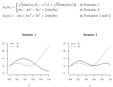
The following simulation study considers two different data generating processes (Scenarios 1 and 2). In both scenarios there are K = 2 parameter regimes and we set αt = A1 if

t _∈G1 =_{1, . . . , T /2_} and αt=A2 if t ∈G2 ={T /2 + 1, . . . , T}, where

A1(u) =

(√

2 sin(πu/2)₋u3_{/2 +}√_{18 sin(3πu/2) in Scenario 1}

8u₋4u2 _−5u3_{+ 2 sin(8u) in Scenario 2}

A2(u) = ₋2u+ 8u2+ 5u3+ 2 sin(8u) in Scenarios 1 and 2.

0.0 0.2 0.4 0.6 0.8 1.0

−5

0

5

10

15

Scenario 1

u A1

A2

0.0 0.2 0.4 0.6 0.8 1.0

−5

0

5

10

15

Scenario 2

u A1

A2

The graphs of the parameter functions are shown in Figure 1. Note that the distance between the regime specific slope functions A1 and A2 is smaller in Scenario 2 than in

Scenario 1, which makes Scenario 2 the more challenging one.

For both scenarios we set βt = 5 sin(t/π) and µt = 5 cos(t/π). We simulate the

re-gressor zit and the error term ǫit according to zit ∼ N(0,1) and ǫit ∼ N(0,1). The

trajectories Xit are obtained as Xit(u) = P_j20₌₁θit,jφj(u) with independent scores θit,j ∼ N (0,[(j₋1/2)π]−2_{) and eigenfunctions φ}

j(u) = √

2 sin((j₋1/2)πu). In order to imple-ment the procedure we evaluate the trajectories on an equidistant grid with 30 grid points in the unit interval. For the choice of the tuning parameters, mt, τnT, and ˜mk we proceed

as described in Section 5. For selecting the threshold τnT we set α = 0.99.

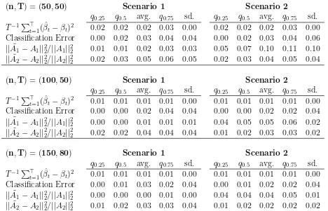
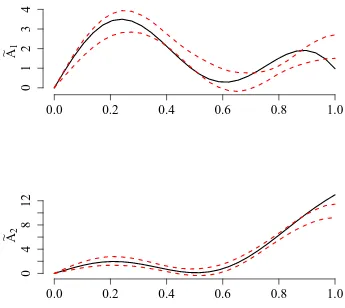
(n,T) = (50,50) Scenario 1 Scenario 2

q0.25 q0.5 avg. q0.75 sd. q0.25 q0.5 avg. q0.75 sd. T−1P⊤

t=1( ˆβt−βt)2 0.02 0.02 0.02 0.03 0.00 0.02 0.02 0.02 0.03 0.00

Classification Error 0.00 0.02 0.03 0.04 0.04 0.00 0.02 0.03 0.04 0.06

||A1˜ ₋A1_||2

2/||A1||22 0.01 0.01 0.02 0.03 0.03 0.05 0.07 0.10 0.11 0.10 ||A2˜ −A2||2

2/||A2||22 0.02 0.03 0.05 0.06 0.05 0.02 0.03 0.04 0.05 0.04

(n,T) = (100,50) Scenario 1 Scenario 2

q0.25 q0.5 avg. q0.75 sd. q0.25 q0.5 avg. q0.75 sd. T−1P⊤

t=1( ˆβt−βt)2 0.01 0.01 0.01 0.01 0.00 0.01 0.01 0.01 0.01 0.00

Classification Error 0.00 0.00 0.02 0.04 0.04 0.00 0.00 0.02 0.02 0.04

||A1˜ −A1||2

2/||A1||22 0.00 0.00 0.01 0.01 0.01 0.04 0.05 0.05 0.06 0.02 ||A2˜ −A2||2

2/||A2||22 0.02 0.02 0.04 0.04 0.04 0.01 0.02 0.03 0.03 0.02

(n,T) = (150,80) Scenario 1 Scenario 2

q0.25 q0.5 avg. q0.75 sd. q0.25 q0.5 avg. q0.75 sd. T−1P⊤

t=1( ˆβt−βt)2 0.01 0.01 0.01 0.01 0.00 0.01 0.01 0.01 0.01 0.00

Classification Error 0.00 0.01 0.03 0.02 0.04 0.00 0.01 0.02 0.02 0.04

||A1˜ −A1||2

2/||A1||22 0.00 0.00 0.00 0.01 0.00 0.04 0.04 0.04 0.05 0.01 ||A2˜ −A2||2

2/||A2||22 0.01 0.02 0.03 0.03 0.04 0.01 0.02 0.02 0.02 0.02

Table 1: The quantities q0.25, q0.5, q0.75, “avg.”, and “sd.” denote the 25% 50% and 75%

quantiles, the arithmetic mean, and the standard deviation of the empirical distribution over Monte Carlo samples.

parameters A1 and A2 is smaller and T is of the same magnitude as n. The simulation is implemented using the statistical software package R (R Core Team, 2017) and the corresponding R-code can be obtained from the authors.

7

Regime Dependent Pricing of Idiosyncratic Risk

Emerging from the influential work of Ang et al. (2006) a considerable number of studies confirm a negative cross-sectional correlation between idiosyncratic volatility and stock returns (see, for instance, Fu, 2009, Hou and Loh, 2016, and references therein). This finding is denoted as the “idiosyncratic volatility puzzle”, since asset pricing theory suggests an opposite outcome. Either investors’ portfolios are well diversified in equilibrium or investors are underdiversified. In the first case, idiosyncratic risk is diversified and the only risk to be priced is systematic. In the second case, idiosyncratic risk matters and investors with standard risk-return preferences asked for a premium to compensate for bearing risk. Starting from theory it would thus be most reasonable to expect either no relation between idiosyncratic volatility and stock returns or a positive relation. As demonstrated in Hou and Loh (2016) this idiosyncratic volatility puzzle has, to a substantial extent, remained unsolved.

In the literature, the idiosyncratic volatility puzzle is typically considered using an ag-gregated monthly perspective. In contrast, we consider the cross-sectional relations between daytime returns yit ∈ R of assets i = 1, . . . , n and the non-aggregated daily idiosyncratic

volatility curves Xit ∈L2([0,1]), where the interval [0,1] describes the standardized

(con-tinuous) intra-day trading time with “0” denoting the start and “1” denoting the end of the intra-day trading. Like Ang et al. (2006), who allow for time varying volatility premiums by conducting separate regressions for each considered month, we allow for daily vary-ing volatility premiums by allowvary-ing for daily varyvary-ing parameters in the followvary-ing partial functional panel regression model:

yit =µt+

Z 1

0

αt(s)Xit(s)ds+βt⊤zit+ǫit, (4)

where µt ∈ R is a daily fixed effect, αt ∈ L2([0,1]) denotes the time varying parameter

function describing the marginal pricing of the idiosyncratic volatility curveXit∈L2([0,1])

at dayt, andβt∈RP is a time varying parameter describing the effect of additional control

variables zit ∈RP. The statistical error term ǫit is a classical scalar error term with finite

but potentially time heteroscedastic variances. We postulate that there are only K < T

different risk regimes G1, . . . , GK collecting identical parameter functions αt. As above,

the common slope function of regime k is denoted by Ak.

FollowingFu(2009), we define the dependent variable as the daytime log-returnsyit :=

log(Pit(1)/Pit(0)), where Pit(0) and Pit(1) denote the opening and closing price of asset i

at day t. As control variable zit ∈ R we use the daily bid-ask spreads which serve as a

proxy for liquidity risk—an important pricing-relevant factor (seeHou and Loh,2016, and references therein).

over full T = 136 trading days between June 3, 2016, and December 15, 2016. The observed intra-day stock prices Pit(sj),j = 1, . . . , J, are defined as the last recorded prices

within standardized 10 minute intervals [sj−1, sj] with s0 = 0, sJ = 1 and equidistant

interval lengths sj −sj−1 = ∆ such that J∆ = 1, where J = 39. For the below described

construction of the idiosyncratic volatility curves Xit(.) we make use of the Fama-French

factors. The Fama-French factors were downloaded from Kenneth French’s homepage3_{; all} other data were gathered from Bloomberg.

Preprocessing. For constructing the idiosyncratic volatility curves Xit(.) we use the

method proposed in M¨uller et al. (2011) with a straightforward adaption to our con-text for estimating idiosyncratic volatility curves instead of total volatility curves. M¨uller et al. (2011) propose estimating the total volatility curve of asset i at day t via smooth-ing the scatter-points ( ˜Yit,j, sj), j = 1, . . . , J, where ˜Yit,j := log(∆−1Yit(sj)2) + q0 is a

scaled and logarithmized version of the squared intra-day returns Yit(sj)2 with Yit(sj) :=

log(Pit(sj)/Pit(sj−1)). The constant q0 = 1.27 is necessary for re-centering the involved

error term (see M¨uller et al., 2011, for technical details). We follow their approach, but instead of using the total intra-day returns Yit(sj),j = 1, . . . , J, which lead to an estimate

of the total volatility curve, we use only theidiosyncratic componentsY∗

it(sj),j = 1, . . . , J,

which leads to an estimate of the idiosyncratic volatility curve Xit(.). For computing the

idiosyncratic intra-day returns Y∗

it(sj), we follow the usual approach and correct the

to-tal intra-day returns Yit(sj) for their systematic market component by regressing them on

the three Fama-French factors (see Fama and French, 1995). We do so by estimating the following functional Fama-French regression model originally proposed by Kokoszka et al.

(2014):

Yit(sj) =b0,it(sj) +b1,it·Mt(sj) +b2,it·St+b3,it ·Ht+uit(sj), j = 1, . . . , J, (5)

where Mt(sj) is the intra-day S&P500 market return, St denotes the “small minus large”

factor, and Ht the “high minus low” factor. St describes the difference in returns between

portfolios of small and large stocks andHtdescribes the difference in returns between

port-folios of high and low book-to-market value stocks. For estimating the model parameters in (5) we use the least-squares estimators proposed by Kokoszka et al. (2014). The id-iosyncratic intra-day returns are then defined as Y∗

it(sj) := ˆb0,it(sj) + ˆuit(sj), where ˆb0,it(sj)

denotes the fitted functional intercept parameter of the (i, t)th regression and ˆuit(s) are

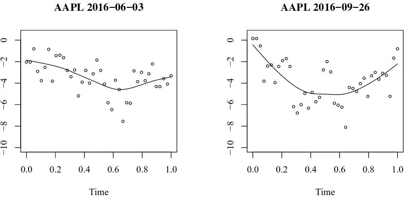
the corresponding regression residuals. Table2provides summary statistics for our sample. Figure 2 shows the idiosyncratic volatility curvesXit, along with their raw-scatter points,

for the Apple stock at two randomly selected trading days.

Remark. Applying the method of M¨uller et al. (2011) in order to estimate the idiosyn-cratic volatility curves Xit from the idiosyncratic intra-day returns Yit∗(sj), j = 1, . . . , J,

leads to “volatility curves” that have to be considered as logarithmized squared volatility curves (see Eq. (9) in M¨uller et al.,2011). Both transformations (taking squares and logs) are monotonic which preserves the sign of our parameter estimates for αt. Furthermore,

working with log-transformed volatility objects is generally advisable, since the original volatilities are known to be heavily skewed (see, for instance, Herskovic et al., 2016).

3

q0.05 q0.25 q0.5 q0.75 q0.95 avg. sd. y (in %) -1.74 -0.56 0.01 0.60 1.79 0.02 1.16

R1

0 X(u)du -4.42 -3.72 -3.20 -2.63 -1.64 -3.14 0.85 ||X_||2

2 3.46 7.67 11.02 14.67 20.50 11.39 5.19 z (in %) 0.02 0.02 0.03 0.05 0.09 0.04 0.03

Table 2: Quantiles, means, and standard deviations of the considered variables.

●●

Figure 2: Idiosyncratic volatility curvesXit and raw scatter points for the Apple Inc. stock

(AAPL) at two randomly selected trading days.

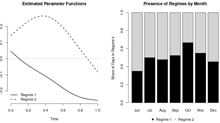
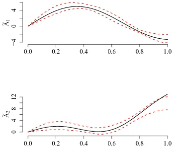
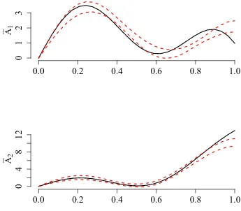
The estimation of model (4) proceeds as described in Section 3. Using our estimation algorithm, we find a number of ˆK = 2 regimes, where each regime contains about the same number of days (see right panel in Figure 3). The left panel in Figure 3 shows the estimated regime specific slope functions ˜A1 and ˜A2. In order to examine how idiosyncratic

volatility is priced in the daytime returns, we consider “marginal effects” defined according to R₀1A˜k(u)du, k = 1,2. For the first regime this marginal effect is clearly negative, for

the second one clearly positive. Our classification thus separates trading days revealing an idiosyncratic volatility puzzle from days which are conform with asset pricing theory. Both parameter functions, however, indicate that the intensity of the pricing varies over trading time within a day.

0.0 0.2 0.4 0.6 0.8 1.0

−0.2

−0.1

0.0

0.1

0.2

Estimated Parameter Functions

Time Regime 1

Regime 2

Jun Jul Aug Sep Oct Nov Dec

Presence of Regimes by Month

Share of Da

ys in Regime k

0.0

0.2

0.4

0.6

0.8

1.0

Regime 1 Regime 2

Figure 3: Estimated regime specific slope functions ˜A1 and ˜A2 (left panel) and marginal effect of idiosyncratic volatility (right panel).

8

Conclusion

In this paper we present a novel regression framework, which allows us to examine regime specific effects of a random function on a scalar response in the presence of a multivariate regressor and time fixed effects. The suggested estimation procedure is designed for a panel data context. We prove consistency of the estimators including rates of convergence and address the practical choice of the tuning parameters involved. In summary, our framework offers a very flexible and data-driven way of assessing heterogeneity in large panels. Our model could be extended in multiple directions for further research. For instance, establishing a connection to the work ofSu et al.(2016) would allow us to identify latent group structures in addition to identifying latent time-regime structures.

The statistical model is motivated by our real data application, where we explore a phenomenon referred to as the idiosyncratic volatility puzzle and search for the presence of such a puzzle in a large panel of US stock prices. Our method allows us to separate puzzling days from non-puzzling days and reveals a much more heterogeneous pricing of idiosyncratic risk than suggested by the monthly analyses in the literature.

References

Ahn, S. C. and A. R. Horenstein (2013). Eigenvalue ratio test for the number of factors.

Aneiros-P´erez, G. and P. Vieu (2006). Semi-functional partial linear regression. Statistics & Probability Letters 76(11), 1102–1110.

Aneiros-P´erez, G. and P. Vieu (2008). Nonparametric time series prediction: A semi-functional partial linear modeling. Journal of Multivariate Analysis 99(5), 834–857.

Aneiros-P´erez, G. and P. Vieu (2013). Testing linearity in semi-parametric functional data analysis. Computational Statistics 28(2), 413–434.

Ang, A., R. J. Hodrick, Y. Xing, and X. Zhang (2006). The cross-section of volatility and expected returns. The Journal of Finance 61(1), 259–299.

Cali´nski, T. and J. Harabasz (1974). A dendrite method for cluster analysis. Communica-tions in Statistics 3(1), 1–27.

Ding, H., Y. Liu, W. Xu, and R. Zhang (2017). A class of functional partially linear single-index models. Journal of Multivariate Analysis 161, 68–82.

Fama, E. F. and K. R. French (1995). Size and book-to-market factors in earnings and returns. The Journal of Finance 50(1), 131–155.

Ferraty, F. and P. Vieu (2006). Nonparametric Functional Data Analysis: Theory and Practice (1. ed.). Springer Series in Statistics. Springer.

Fu, F. (2009). Idiosyncratic risk and the cross-section of expected stock returns. Journal of Financial Economics 91(1), 24–37.

Hall, P. and J. L. Horowitz (2007). Methodology and convergence rates for functional linear regression. The Annals of Statistics 35(1), 70–91.

Herskovic, B., B. Kelly, H. Lustig, and S. Van Nieuwerburgh (2016). The common factor in idiosyncratic volatility: Quantitative asset pricing implications. Journal of Financial Economics 119(2), 249–283.

H¨ormann, S. and P. Kokoszka (2010). Weakly dependent functional data. The Annals of Statistics 38(3), 1845–1884.

Horv´ath, L. and P. Kokoszka (2012). Inference for Functional Data with Applications (1. ed.). Springer Series in Statistics. Springer.

Horv´ath, L. and R. Reeder (2012). Detecting changes in functional linear models. Journal of Multivariate Analysis 111, 310–334.

Hou, K. and R. K. Loh (2016). Have we solved the idiosyncratic volatility puzzle? Journal of Financial Economics 121(1), 167–194.

Kokoszka, P., H. Miao, and X. Zhang (2014). Functional dynamic factor model for intraday price curves. Journal of Financial Econometrics 13(2), 456–477.

Kong, D., K. Xue, F. Yao, and H. H. Zhang (2016). Partially functional linear regression in high dimensions. Biometrika 103(1), 147–159.

Lian, H. (2011). Functional partial linear model.Journal of Nonparametric Statistics 23(1), 115–128.

Lu, Y., J. Du, and Z. Sun (2014). Functional partially linear quantile regression model.

Metrika 77(2), 317–332.

M¨uller, H.-G., R. Sen, and U. Stadtm¨uller (2011). Functional data analysis for volatility.

Journal of Econometrics 165(2), 233–245.

Peng, Q.-Y., J.-J. Zhou, and N.-S. Tang (2016). Varying coefficient partially functional linear regression models. Statistical Papers 57(3), 827–841.

R Core Team (2017). R: A Language and Environment for Statistical Computing. Vienna, Austria: R Foundation for Statistical Computing.

Ramsay, J. O. and B. W. Silverman (2005). Functional Data Analysis (2. ed.). Springer Series in Statistics. Springer.

Reiss, P. T., J. Goldsmith, H. L. Shang, and R. T. Ogden (2016). Methods for scalar-on-function regression. International Statistical Review.

Schipper, M., J. M. Taylor, and X. Lin (2008). Generalized monotonic functional mixed models with application to modelling normal tissue complications. Journal of the Royal Statistical Society: Series C (Applied Statistics) 57(2), 149–163.

Shin, H. (2009). Partial functional linear regression. Journal of Statistical Planning and Inference 139(10), 3405–3418.

Shin, H. and M. H. Lee (2012). On prediction rate in partial functional linear regression.

Journal of Multivariate Analysis 103(1), 93–106.

Su, L., Z. Shi, and P. C. Phillips (2016). Identifying latent structures in panel data.

Econometrica 84(6), 2215–2264.

Tang, Q. and L. Cheng (2014). Partial functional linear quantile regression. Science China Mathematics 57(12), 2589–2608.

Vogt, M. and O. Linton (2017). Classification of non-parametric regression functions in longitudinal data models. Journal of the Royal Statistical Society: Series B (Statistical Methodology) 79(1), 5–27.

Wang, G., X.-N. Feng, and M. Chen (2016). Functional partial linear single-index model.

Zhang, D., X. Lin, and M. Sowers (2007). Two-stage functional mixed models for evaluating the effect of longitudinal covariate profiles on a scalar outcome. Biometrics 63(2), 351– 362.

Supplemental Paper for:

Parameter Regimes in Partial Functional

Panel Regression

by Dominik Liebl and Fabian Walders

In part A of this supplement we provide formal proofs for Theorems 4.1, 4.2, and 4.3

as well as Lemma 4.1. Further, we briefly discuss the properties of the threshold τnT as

suggested in Section 5. In part B, we provide additional results from our simulation study.

Throughout this supplement we use the symbols C and c to denote positive constants. Their precise meaning varies in many cases from term to term.

A

Proofs

In this section we use the following notation for norms in addition to the ones introduced in the main body of the paper. Given some f1 ∈L2_{([0,1]) and a mappingF1 :L}2_([0,1])→R,

we use as norm of F1 the operator norm ||F1||H′ := sup_||f

1||2=1|F1(f1)|. Further, for an

integral operator F2 : L2_{([0,1]) → L}2_{([0,1]) with kernel f2 ∈ L}2_{([0,1]×[0,1]), denote}

its Hilbert-Schmidt norm as ||F2||S := ||f2||2, where in this case || · ||2 is the L2 norm in L2_{([0,1]×[0,1]).}

For the sake of readability we will proof the Lemma and Theorems forP = 1, while the generalization toP >1 is straightforward and does not add any additional insights. In this spirit we ease notation by dropping boldface notation and the dependence on coordinate labels p. Now, turning to a formal argumentation, we begin collecting a number of basic results readily available in the functional data literature. Provided Assumption 1 holds, the sequence _{(zit, Xit) : 1≤i≤n}is iid with finite fourth moments for every 1≤t ≤T.

Moment calculations as well as the results in, e.g., H¨ormann and Kokoszka (2010) imply for any 1≤t≤T asn → ∞ that

EKˆzX,t−KzX,k

2

2

=O(n−1) (6)

EKˆz,t−Kz,k

2

=O(n−1) (7)

EKˆX,t−KX,k

2

2

E[|z¯t−E[zit]|2] =O(n−1)

E[X¯_t−E[X_it]2

2] =O(n

−1_),

E[_||KˆXǫ,t||22] =O(n−1)

E[|Kˆzǫ,t|2] =O(n−1).

Denote the Hilbert-Schmidt norm of the distance between t-wise empirical covariance operator and population covariance operator asDt :=||Γˆt−Γk||S. Note that for anyj ≥1, |λˆj,t −λj,k| ≤ Dt. Since E[Dtq] = O(n−q/2) for q = 1,2, . . . (provided sufficiently high

moments exist) it holds that

Ehλˆj,t−λj,k

qi

=O(n−q/2) q = 1,2. . . (8)

for j ≥1. In contrast to Shin (2009) the estimators ˆβt and ˆaj,t are calculated on the basis

of empirically centered data. As, however, the arguments in Hall and Horowitz (2007) are formulated in terms of empirically centered variables as well, the argument in Shin (2009) allows to conclude immediately that for any 1≤t≤T

||Φˆt−Φk||2H′ =

m

X

j=1

hKˆzX,t,φˆj,ti

ˆ

λj,t

ˆ

φj,t− ∞

X

j=1

hKzX, φji

λj

φj

2

2

=Op(n

1−2ν

µ+2ν), (9)

where we denote mt=m for simplicity.

A.1

Proof of Theorem

4.1

For any 1 _≤t_≤T the estimator ˆβt can be written as

ˆ

βt = ˆBt−1[ ˆKzy,t−Φˆt( ˆKXy,t)]

with ˆBt := [ ˆKz,t−Φˆt( ˆKzX,t)]. Regarding the inverse note that it follows from (6), (7), and

(9) that

ˆ

Bt:= [ ˆKz,t−Φˆt( ˆKzX,t)]→P [Kz,k−Φk(KzX,k)] =:Bk

as n_{→ ∞}, which certainly implies ˆB−1

t =B−1+op(1).

As in Shin (2009), we split the term [ ˆKzy,t−Φˆt( ˆKXy,t)] =R0,1,t+R0,2,t +R0,3,t, while

her argument allows to immediately conclude

R0,1,t :=n−1 n

X

i=1

(zc

it−Φk(Xitc))ǫitc =Op(n−1/2)

R0,2,t :=n−1 n

X

i=1

However, for the remaining term we approach in a different manner:

|R0,3,t|:=|n−1 n

X

i=1

(zc

it−Φˆt(Xitc))hXitc, αti|

≤ |hKˆzX,t−KzX, αti|+|hKzX, αti −n−1 n

X

i=1

ˆ

Φt(Xitc)hXitc, αti|

≤R1,1,t+R1,2,t

with R1,1,t and R1,2,t defined as follows.

R1,1,t :=|hKˆzX,t−KzX, αti| ≤ ||αt||2||KˆzX,t−KzX||2

=Op(n−1/2)

as a consequence of (6). The second term is defined as

R1,2,t :=|hKzX,k, αti −n−1 n

X

i=1

ˆ

Φt(Xitc)hXitc, αti|

≤R2,1,t+R2,2,t,

with

R2,1,t :=| ∞

X

j=m+1

hKzX,k, φj,kia∗j,k|

R2,2,t :=| m

X

j=1

hKzX,k, φj,kia∗j,k − m

X

j=1

hKˆzX,t,φˆj,tiˆaj,t|,

where we used a∗

j,t :=hαt, φj,ki.4 For the first term observeR2,1,t =O(n

1−µ−2ν

µ+2ν ) =O(n−1/2). The second one can be split in three parts

R2,2,t ≤R3,1,t+R3,2,t+R3,3,t

with

R3,1,t := m

X

j=1

||KˆzX,t−KzX,k||2(||φˆj,t−φj,k||2)||αt||2 +a∗j,t) = Op(n−1/2),

R3,2,t :=||αt||2

m

X

j=1

hKzX,k, φj,ki||φˆj,t−φj,k||2 =Op(n−1/2)

and

R3,3,t :=||KzX,k||2||αt||2

m

X

j=1

||φˆj,t−φj,k||22+||KzX,k||2

m

X

j=1

||φˆj,t−φj,k||2|a∗j,t|.

4

Bounds on||φˆj,t−φj,k||22 can be obtained using the techniques inHall and Horowitz(2007).

For this purpose, define the following events:

1. F1,m,t :={Cn

2(1+µ)

µ+2ν D2

t ≤1/2}

2. F2,m,t :={|λˆj,t−λl,k|−2 ≤4|λj,k −λl,k|−2 ≤Cn

2(1+µ)

µ+2ν }. 3. F3,m,t :=F1,m,t∩F2,m,t

Note thatP(Fc

1,m,t) = o(1) as well asP(F2c,m,t) = o(1) due root-nconsistency of the empirical

covariance operator and its corresponding eigenvalues. It is shown that this property holds uniformly over 1 ≤ t ≤ T as (n, T) → ∞ in the Proof of Lemma 1 below. The second event is borrowed from Hall and Horowitz (2007), while the first one allows to conclude that1(F1,m,t)(1−Cn

2(1+µ)

µ+2ν D2

t)−1 ≤2 for a suitably chosen constantC. This in turn implies

that the bound on_||φˆj,t−φj,k||22 inHall and Horowitz(2007) reads onF3,m,tgiven a suitable

constant C in F1,m,t as follows.

E[1(F3,m,t)||φˆj,t−φj,k||22]

≤16E

" X

l:l6=j

(λj,k−λl,k)−2

Z 1

0

Z 1

0

( ˆKX,t(u, v)−KX,k(u, v))φj,k(u)φl,k(v)dudv

2#

=O(n−1j2),

where 1 _≤j _≤m. This in turn allows to conclude for the first summand in R3,3,t,

1(F3,m,t)||KzX,k||2||αt||2

m

X

j=1

||φˆj,t−φj,k||22 =Op(n−1m3)

=Op(n

3−µ−2ν

µ+2ν ) =Op(n−1/2)

due to Assumption 4. The second summand in R3,3 behaves according to

1(F3,m,t)||KzX,k||2

m

X

j=1

||φˆj,t−φj,k||2|aj,t∗ |=Op(n−1/2)

again using Assumption 4. Since P(Fc

3,m,t)≤P(F1c,m,t) +P(F2c,m,t) = o(1) as claimed before,

it follows R3,3,t =Op(n−1/2). Combining arguments implies ˆβt−βt = Op(n−1/2) for every

1 ≤t ≤ T, which concludes the Proof the first result in Theorem 4.1. Turning to ˆαt note

that

||αˆt−αt||22 ≤

m

X

j=1

(ˆaj,t−a∗j,t)2+m m

X

j=1

a∗_j,t||φˆj,t−φj,k||22+ ∞

X

j=m+1

The results in Hall and Horowitz(2007) and Shin (2009) immediately translate to

mPm_j=1(a∗

j,t)2||φˆj,t−φj,k||22 and

P∞

j=m+1a∗j,t which are bothOp(n

1−2ν

µ+2ν). The remaining term can be split according to

m

X

j=1

(ˆaj,t−a∗j,t)2 ≤2 m

X

j=1

(ˆλj,thKˆyX,t# −βˆtKˆzX,t# ,φˆj,ti −a∗j,t)2+ 2 m

X

j=1

(ˆλj,thry,trx,t−βˆtrz,trX,t,φˆj,ti)2

(10)

with K_yX,t# := n−1Pn

i=1(yit−E[yit])(Xit−E[Xit]), K #

zX,t := n−1

Pn

i=1(zit −E[zit])(Xit− E[Xit]), rx,t :=E[Xit]−X¯t, ry,t:=E[yit]−y¯t andrz,t :=E[zit]−z¯t. Note that,||rx,t||2, ry,t

andrz,tare all errors from parametric estimation problems and thus of ordern−1/2. Bounds

on ˆλj,t−λj,k as well as||φˆj,t−φj,k||are asymptotically equivalent for data centered around

their arithmetic mean and data centered around their population expectation. Together with the above arguments showing ˆβt −βt = Op(n−1/2), it follows that the first term

in (10) is asymptotically equivalent to the corresponding term in Shin (2009), implying

Pm

j=1(ˆλj,thKˆ #

yX,t−βˆtKˆzX,t# ,φˆj,ti −a∗j,t)2 =Op(n

1−2ν

µ+2ν). Now, define the event

F4,m,t:={|λˆj,t−λj,k|< λj/2 : 1≤j ≤m}

on which the second term in (10) behaves according to

1(F4,m,t) m

X

j=1

(ˆλj,thry,trX,t−βˆtrˆz,trX,t,φˆj,ti)2 ≤8 m

X

j=1

λ2_j,tr_y,t2 _||rX,t||22+ 8

m

X

j=1

λ2_j,tβˆ_t2r2_z,t||rX,t||22

=Op(n

1+2µ−2µ−4ν

µ+2ν ) =O

p(n

1−2ν

µ+2ν) since P(Fc

4,m,t) =o(1)∀t asn → ∞as a consequence of (8). Finally, combining arguments

yields ||αˆt−αt||22 =Op(n

1−2ν

µ+2ν) for any 1≤ t≤T as n → ∞, which concludes the proof of the second part of Theorem 4.1.

A.2

Proof of Lemma

4.1

In what follows we ultimately show that the quantities ˆα∆

t are consistent for α∆t in the L2

norm, uniformly over 1 ≤ t≤ T. This in turn implies classification consistency as will be shown in the proof of Theorem 4.2. The remaining parts of the Lemma are shown on the way, as they are required to obtain the result concerning ˆα∆

t .

We begin listing a number of basic observations, which are a consequence of the iid sampling scheme in the cross-section as well as stationarity of the regressors and the error over time within regimes. We also use the results inHall and Horowitz(2007) andH¨ormann and Kokoszka (2010).

• Note that since _{Xit : t ∈ Gk, 1 ≤ i ≤ n} is stationary, E[Dt2] does not vary in

conclude

• Empirical variances of zit and ǫit behave according to

P

• The empirical covariances between regressors and error in any cross-section are de-noted ˆKXǫ,t :=n−1Pn_i=1Xitcǫcit and ˆKzǫ,t :=n−1P_in₌₁zitcǫcit. In analogy to before

in-Similar arguments can be used to show

P( max

1≤t≤T|

ˆ

Kzǫ,t|2 > c) =O(nδ−1) +O(nδ−2) = o(1). (13)

• Uniform consistency of the empirical covariance ˆKzX,t(u) can be shown with similar

P( max

1≤t≤T||

ˆ

KzX,t−KzX,k||22 > c)

≤ K

X

k=1

X

t∈Gk

P

||Kˆ_zX,t# −KzX,k||22 > c/4

+

K

X

k=1

X

t∈Gk

P ||rX,t||22rz,t2 > c/4

≤K max

1≤k≤K|Gk|

n−1_E[||(z

it−E[zit])(Xit−E[Xit])−KzX,k||22] c

+K max

1≤k≤K|Gk|

E[_|z¯t−E[zit]|2]E

||X¯t−E[Xit]||22

c

=O(nδ−1) +O(nδ−2) = o(1). (14)

For the following proof it will be necessary to obtain uniform consistency ofPm_j=1λ−_j,k2||φj,k−

ˆ

φj,t||22. For this purpose observe that ˆλj,t ≥ λj,t/2 for 1 ≤ j ≤ m on on F4,m,t. Further,

provided that F3,m,t holds for any 1 ≤ t ≤ T, observe that E[||φˆj,t−φj,t||22] = O(n−1j2)

uniformly on 1 _≤ j _≤ m. Note that the results in Hall and Horowitz (2007) imply that uniformly on j and l

nE

"Z 1

0

Z 1

0

( ˆKX,t(u, v)−KX,k)(u, v))φj,k(u)φl,k(v)dudv

2#

≤λj,kλl,k

as well as

E

" X

l:l6=j

(λj,k −λl,k)−2

Z 1

0

Z 1

0

( ˆKX,t(u, v)−KX,k(u, v))φj,k(u)φl,k(v)dudv

2#

=O(n−1j2),

uniformly on 1≤j ≤m. Further observe that

E[1(F3,m,t)||φˆj,t−φj,k||22]

≤16E

" X

l:l6=j

(λj,k−λl,k)−2

Z 1

0

Z 1

0

( ˆKX,t(u, v)−KX,k(u, v))φj,k(u)φl,k(v)dudv

2#

=O(n−1_j2_).

In order to proceed introduce the event

• F5,m,t :={|λˆj,t−λj,k| ≥ 1₄|λj,k −λl,k|: 1≤j ≤m}.

Observe for the events_F1,m,t,F2,m,t,F4,m,t and F5,m,t the following. Note for

Kmax1≤k≤K|Gk|P(F1c,m,t), that

K max

1≤k≤K|Gk|P(Cn

2(1+µ)

µ+2ν D2

t >1/2)≤K max

1≤k≤K|Gk|

n2(1+µ+2µν)E[D2

t]

2C

for any C > 0. Further it holds thatKmax1≤k≤K|Gk|P(F1c,m,t) = o(1) as (n, T)→ ∞.

K max

1≤k≤K|Gk|P(F c

2,m,t) = K max

1≤k≤K|Gk|P(∃1≤j ≤m: |

ˆ

λj,t−λl,k|−2 >4|λj,k−λl,k|−2)

=K max

1≤k≤K|Gk|P(∃1≤j ≤m: |

ˆ

λj,t−λl,k|<

1

2|λj,k −λl,k|)

≤K max

1≤k≤K|Gk|P(∃1≤j ≤m: |

ˆ

λj,t−λj,k|>

1

2|λj,k−λl,k|)

≤K max

1≤k≤K|Gk|P(Dt>

1

2min{λj,k−λl,j+1, λj−1,k−λl,j})

≤K max

1≤k≤K|Gk|

CE[_D2

t]

min_{λj,k−λl,j+1, λj−1,k −λl,j}2

=O(nδn−1m2(1+µ)) =o(1)

by the fact that _Dt ≥ |ˆλj,t−λj,k| and Assumptions 2 and 4. Beyond that it holds

K max

1≤k≤K|Gk|P(F c

4,m,t)≤K max

1≤k≤K|Gk|P

sup

1≤j≤m|

ˆ

λj,t−λj,k|>

1 2λm,k

≤K max

1≤k≤K|Gk|P

Dt>

1 2λm,k

≤K max

1≤k≤K|Gk|

4E[_D2

t]

λ2

m,k

=O(nδnµµ−+22νν) = o(1). Combining arguments leads to

P max

1≤t≤T m

X

j=1

ˆ

λ−_j,t2_||φj,k−φˆj,t||22 > c

!

≤K max

1≤k≤K|Gk|

Pm j=1λ

−2

j,kE[1(F3,m,t)||φˆj,t−φj,k||22]

C +K1max≤k≤K|Gk|(P(F c

1,m,t) +P(F2c,m,t) +P(F4c,m,t))

=O(n3+(1+δµ)µ+2−ν2(1−δ)ν) +o(1)

=o(1) (15)

Note that this result implies in particular that

P max

1≤t≤T m

X

j=1

||φj,k−φˆj,t||22 > c

!

=o(1),

which will be used without further reference in what follows. For later purpose, define the event St according to

St:=

σˆ_ǫ,t2 −σ_ǫ,k2 ≤ 1

2σ

2

ǫ,k : 1≤j ≤m

It will be shown in a moment that also PT_t=1P(Sc

t) = o(1). However this requires some

preparation since ˆσ2

ǫ,t includes estimation errors from ˆβt and ˆαt. We thus begin by showing P(max1≤t≤T |βˆt−βt|> c) = o(1). The estimator ˆβt makes multiple use of the operator ˆΦt,

which can, starting from the Riesz-Frechet representation Theorem (see Shin (2009)), be handled according to

, which is independent of

tando(1) because the truncation parameter diverges at infinity and henceR4,3is arbitrarily

small fornlarge enough. The remaining summands are defined and treated as follows. The first one behaves according to

R4,1,t :=

The three summands behave as follows:

P

For uniform consistency of ˆβt it remains to show that

• P(max1≤t≤T |R0,1,t|> c) =o(1),

• P(max1≤t≤T |R0,3,t|> c) =o(1).

For this purpose consider

P max

1≤t≤T|n

−1

n

X

i=1

(zc_it−Φ(X_itc))ǫc_it|> c

!

≤K max

1≤k≤K

P(|Kˆzǫ,t|> c/2) +P(||Φk||H′|Kˆ_ǫX,t|> c/2)

=o(1)

due to (12) and (13). Further note for R0,2,t

P

max

1≤t≤T|Φ( ˆKǫX,t)−

ˆ

Φt( ˆKǫX,t)|

≤K max

1≤k≤KP(||

ˆ

Φt−Φk||H′|Kˆ_ǫX,t|> c)

≤K max

1≤k≤K|Gk|P(

||KǫX,k||2||Φˆt−Φk||H′

> c)

+K max

1≤k≤K|Gk|P(||

ˆ

KǫX,t−KǫX,k||22 > c)

=o(1)

as a consequence of (12) and (16). For the remaining terms, argue along the same lines as in the Proof of Lemma 1:

P( max

1≤t≤T|R0,3,t|> c) := P( max1≤t≤T|R1,1,t|> c) +P( max1≤t≤T|R1,2,t|> c)

P( max

1≤t≤T|R1,1,t|> c)≤P( max1≤t≤T|||αt||2||

ˆ

KzX,t−KzX||2|> c)

=o(1)

because of (14). As before the remaining term can be bounded according to R1,2,t ≤

R2,1,t+R2,2,t, where the two summands are defined above. WhileR2,1,t =R2,1 =O(n−1/2)

deterministically and independent of t, note for the second bound R2,2,t ≤R3,1,t+R3,2,t+

R3,3,t as before and further:

P( max

1≤t≤T|R3,1,t|> c)≤K1max≤k≤K|Gk|P | m

X

j=1

||KˆzX,t−KzX,k||2(||φˆj,t−φj,k||2)||αt||2+a∗j,t)|> c

!

≤K max

1≤k≤K|Gk|

E[_||KˆzX,t−KzX,k||22]

1

2E[mPm

j=1||φˆj,t−φj,k||221(F3,m,t)]

1 2

c

+K max

1≤k≤K|Gk|

E[||KˆzX,t−KzX,k||22](

Pm j=1a∗j,t)2

c +K1max≤k≤K|Gk|P(F c

3,m,t)

Further for R3,2,t note:

P( max

1≤t≤T|R3,2,t|> c)≤K1max≤k≤K|Gk|P ||αt||2 m

X

j=1

|hKzX,k, φj,k|i||φˆj,t−φj,k||2 > c

!

≤K max

1≤k≤K|Gk|

||Ak||2mPm_j=1|hKzX,k, φj,ki2E

h

||φˆj,t−φj,k||221(F3,m,t)

i

c

+K max

1≤k≤K|Gk|P(F c

3,m,t)

=O(mnδ−1) +o(1) =o(1).

Using similar arguments, one obtains for R3,3,t:

P( max

1≤t≤T|R3,3,t|> c)≤K1max≤k≤K|Gk|P(||KzX,k||2||αt||2 m

X

j=1

||φˆj,t−φj,k||22 > c/2)+

+K max

1≤k≤K|Gk|P(||KzX,k||2 m

X

j=1

||φˆj,t−φj,k||2|a∗j,t|> c/2)

=o(1).

Hence _P(max1≤t≤T( ˆβt−βt)2 > c) = o(1) as claimed in the Lemma. Now, turning to the

estimation error in the functional parameter estimates ˆαt observe that

P( max

1≤t≤T(||αˆt−αt||

2

2 > c)≤K max

1≤k≤K|Gk|P ||αˆt−αt||

2 2 > c

≤R8,1,t+R8,2,t+R8,3,t+R8,4,t.

This is because due to Assumption 2, P∞_j=m+1a∗

j,k2 is a null sequence and hence arbitrarily

small for sufficiently large n. The terms R8,1,t−R8,4,t are defined and treated as follows.

R8,1,t :=K max

1≤k≤K|Gk|P





m

X

j=1

ˆ

λ−2

j,t n−1 n

X

i=1

hXit,φˆj,tiǫit

!2 > c





≤K max

1≤k≤K|Gk|

Pm j=1λ

−2

j,kE

h

||KˆXǫ,t||22

i

c +K1max≤k≤K|Gk|P F c

4,m,t

due to Assumption 4.

tion 2, the first two summands areo(1). As a consequence of (15) the third summand iso(1). Together with the above results this implies R8,2,t = o(1). Further, with aj,t := hαt,φˆj,ti,

behavior of the scaling, which itself is random, needs to be explored. Contributing to this,

by (13) and the above results. Further

R10,1,t :=K max

with R11,1,t−R11,2,t to be treated as follows.

by (11) and the above results. Further it holds that

R11,2,t :=K max

in light of the above results. Combining results yields PK_k=1P_t∈G kP(S

c

t) = o(1). Now,

finally turning to ˆα(∆)_t , for sufficiently largen

P

R12,1,t can be decomposed according to

where, for some suitable c >0,

These terms in turn behave as follows.

R13,1,t ≤K max

with

In order to continue, note that by the mean value Theorem

• it holds on _St that |σˆǫ,t−σǫ,k| ≤ 1₂(σǫ,k/2)−

Following the argument from before (clearly Pm_j=1|a∗ j,k|λ

given δ as in Assumption 3.

as was argued before. It remains to show that R14,2,t =o(1). For this purpose note

R14,2,t =K max

1≤k≤K|Gk|P m

X

j=1

(a∗_j,t−aj,t)2

ˆ

λj,t

ˆ

σ2

ǫ,t

> c

!

≤K max

1≤k≤K|Gk|

Pm

j=1||αt||22E[||φˆj,t−φj,k||221(F3,m,t)] λ2

j

σ2

ǫ

c +K1max≤k≤K|Gk|P F c

4,m,t

+K max

1≤k≤K|Gk|P(S c

t) +K max

1≤k≤K|Gk|P F c

3,m,t

=o(1).

Combining arguments implies the last part of the Lemma.

A.3

Proof of Theorem

4.2

Using the results presented in the previous Lemma it is possible to argue in analogy to the proof of Theorem 3.1 in Vogt and Linton (2017) to proof classification consistency in the sense of our Theorem 4.2. For this purpose consider the set S(j) _{={1, . . . , T} \}S

l<jGˆl at

an iteration step 1 _≤ j _≤ Kˆ ₋1 of the algorithm described in Section 3. For a t _∈ S(j)

denote the set of indexes corresponding to the ordered distances ˆ∆t(1) ≤ · · · ≤∆ˆt(|S(j)_|) as

{(1), . . . ,(_|S(j)_{|)}. In analogy, the index set corresponding ordered population distances}

∆t[1] ≤ · · · ≤ ∆t[|S(j)_|] is denoted as {[1], . . . ,[|S(j)|]}, where ∆_ts is as in Assumption 7.

Now, define an index ˆκ according to ˆ∆t(ˆκ) < τnT < ∆ˆt(ˆκ+1). Beyond that a population

counterpart, κ, obtains as 0 = ∆t[κ]< τnT <∆t[κ+1]. It holds that

P({(1), . . . ,(ˆκ)} 6={([1], . . . ,[κ]})≤P({(1), . . . ,(κ)} 6={[1], . . . ,[κ]}) +P(ˆκ6=κ) (17) =o(1) +o(1) =o(1).

In order to prove that the first probability on the right hand side of (17) is a null sequence, suppose that t _∈ Gk, with 1 ≤ k ≤ K. As indicated, there are κ ≥ 1 indexes in S(j)

being elements of Gk. For the corresponding distances to reference time t it holds that

∆t[1] =· · ·= ∆t[κ]= 0 by definition. The remaining distances are bounded away from zero

by 0< C∆_≤∆t[κ+1]≤ · · · ≤∆t[|S(j)_|] due to Assumption 7.

As shown in the above Lemma, max1≤t≤T||αˆ(∆)t −α

(∆)

t ||22 =op(1) implying that max1≤s≤T |∆ˆts−

∆ts| =op(1) which holds for any reference period t. Combining arguments allows to

con-clude max1≤(s)≤κ∆ˆt(s)=op(1) and minκ<(s)≤|S(j)_|∆ˆ_t(s) ≥C∆+o_p(1) as well as max_1≤[s]≤κ∆ˆ_t[s] =

op(1) and minκ<[s]≤|S(j)_|∆ˆ_t[s] ≥ C_∆+o_p(1). This immediately implies that the first

prob-ability on the right hand side of (17) tends to zero. Further note that the specifica-tion of the threshold in Assumpspecifica-tion 7 immediately implies P

ˆ

∆t[κ] < τnT

→ 1 and

P

ˆ

∆t[κ+1]> τnT

→1 as n _{→ ∞}. As a consequence of this _P∆ˆt[κ] < τnT <∆ˆt[κ+1]

A.4

Remark 1

As a consequence of Theorem4.2, the classification error is, in what follows, asymptotically negligible. To see this note that an analogous argument as in Vogt and Linton(2017) holds in our context: let s1(n, T) and s2(n, T) be two arbitrary sequences such thatsj(n, T)→0

as n, T _{→ ∞} forj = 1,2. Now, note that for any constants M1, M2 >0

P



s1(n, T)X

t∈Gˆk

( ˜βt,k−βt)2 > M1





≤P



  



s1(n, T)X

t∈Gˆk

( ˜βt,k−βt)2 > M1

 

∩ n

ˆ

Gk =Gk

o 

+_P n

ˆ

Gk 6=Gk

o

=P s1(n, T)X

t∈Gk

( ˜β_t,k∗ ₋βt)2 > M1

!

+o(1).

and

P

s2(n, T)||A˜k−Ak||22 > M2

≤P

n

s2(n, T)||A˜k−Ak||22 > M2

o

∩nGˆk=Gk

o

+_PnGˆk 6=Gk

o

=P

s2(n, T)||A˜∗_k−Ak||22 > M2

+o(1).

The quantities ˜β∗

t,k and ˜A∗k are the estimators ˜βt,k and ˜Ak calculated from {(yit, Xit, zit) :

1 _≤ i _≤ n, t _∈ Gk}, i.e. without classification errors. Note in particular that the

depen-dence structure formulated in our assumptions does not disturb this argument.

In light of this remark, the proof of Theorem4.3 starts from the quantities ˜β∗

t,k and ˜A∗k

rather than their contaminated counterparts.

A.5

Remark 2

Denote as ˜φ∗

j,k,˜λ∗j,k,K˜X,k∗ the estimators ˜φj,k,λ˜j,k,K˜X,k from the observations {(zit, Xit) :

1 ≤i ≤ n, t∈ Gk} ). In analogy interpret ˜Φ∗k,K˜zX,k∗ and ˜Kz,k∗ as the estimates ˜Φk,K˜zX,k

and ˜Kz,k without classification error.

Note, that due to Assumption 1 for every regimeGk, the sequence{Xit : 1≤i≤n, t∈

Gk} is L4m-approximable. Thus the following inequalities from H¨ormann and Kokoszka

(2010) hold (where for the third inequality we used our Assumption 2 already).

E

K˜X,k∗ −KX,k

2

2

≤C(n_|Gk|)−1 (18)

Eh

˜λ∗j,k−λj,k

qi