Improved Bayesian Compression
Marco Federici University of Amsterdam [email protected]
Karen Ullrich University of Amsterdam [email protected]
Max Welling University of Amsterdam
Canadian Institute for Advanced Research (CIFAR) [email protected]
1
Variational Bayesian Networks for Compression
Compression of Neural Networks (NN) has become a highly studied topic in recent years. The main reason for this is the demand for industrial scale usage of NNs such as deploying them on mobile devices, storing them efficiently, transmitting them via band-limited channels and most importantly doing inference at scale. There have been two proposals that show strong results, both using empirical Bayesian priors: (i) Ullrich et al. [2017] show impressive compression results by use of an adaptive Mixture of Gaussian prior on independent delta distributed weights. This idea has initially been proposed asSoft-Weight Sharing by Nowlan and Hinton [1992] but was never demonstrated to compress before. (ii) Equivalently, Molchanov et al. [2017] useVariational Dropout[Kingma et al., 2015] to prune out independent Gaussian posterior weights with high uncertainties. To achieve high pruning rates the authors refined the originally proposed approximations to the KL-divergence and a different parametrization to increase the stability of the training procedure. In this work, we propose to join these two somewhat orthogonal compression schemes since (ii) seems to prune out more weights but does not provide a technique for quantization such as (i). We find our method to outperform both of the above.
2
Method
Given a datasetD={xi, yi}Ni=1and a model parametrized by a weight vectorw, the learning goal consists in the maximization of the posterior probability of the parameters given the datap(w|D). Since this quantity involves the computation of intractable integrals, the original objective is replaced with a lower bound obtained by introducing an approximate parametric posterior distributionqφ(w). In theVariational Inferenceframework, the objective function is expressed as aVariational Lower Bound:
L(φ) =
N
X
i=1
Ew∼qφ(w)[logp(yn|xn,w)]
| {z }
LD(φ)
−DKL(qφ(w)||p(w)) (1)
The first termLD(φ)of the equation represents the log-likelihood of the model predictions, while the
second partDKL(qφ(w)||p(w))stands for the KL-Divergence between the weights approximate posteriorqφ(w)and their prior distributionp(w). This term works as a regularizer whose effects on the training procedure and tractability depend on the chosen functional form for the two distributions. In this work we propose the use of a joint distribution over theD-dimensional weight vectorwand their corresponding centersm.
Table 1 shows the factorization and functional form of the prior and posterior distributions. Each conditional posteriorqσi(wi|mi)is represented with a Gaussian distribution with a varianceσ
2
i
around a centermidefined as a delta peak determined by the parameterθi.
Table 1:Choice of probability distribution for the approximate posteriorqφ(w,m)and the prior distribution pψ(w,m).GMψ(mi)represent a Gaussian mixture model overmiparametrized withψ.
Distribution factorization Functional forms qφ(w,m) =
D
Y
i=1
(qσi(wi|mi)qθi(mi))
qσi(wi|mi) =N wi|mi, σ
2
i
qθi(mi) =δθi(mi)
pψ(w,m) =
D
Y
i=1
(p(wi) pψ(mi))
p(wi)∝1/|wi|
pψ(mi) =GMψ(mi)
On the other hand, the joint prior is modeled as a product of independent distributions overw andm. Eachp(wi)represents a log-uniform distribution, whilepψ(mi)is a mixture of Gaussian distribution parametrized withψ that represents theKmixing proportions π, the mean of each Gaussian componentµand their respective precisionλ. In this settings, the KL-Divergence between the prior and posterior distribution can be expressed as:
DKL(qφ(w,m)||pψ(w,m)) =
D
X
i=1
DKL
N wi|θi, σi2
|| 1 |wi|
+ logGMψ(mi=θi)
+C
(2) WhereDKL N wi|θi, σi2
||1/|wi|
can be effectively approximated as described in Molchanov et al. [2017]. A full derivation can be found in appendix C.
The zero-centered heavy-tailed prior distribution onw induces sparsity in the parameters vector, while the adaptive mixture model applied on the weight centersmforces a clustering behavior while adjusting the parametersψto better match their distribution.
3
Experiments
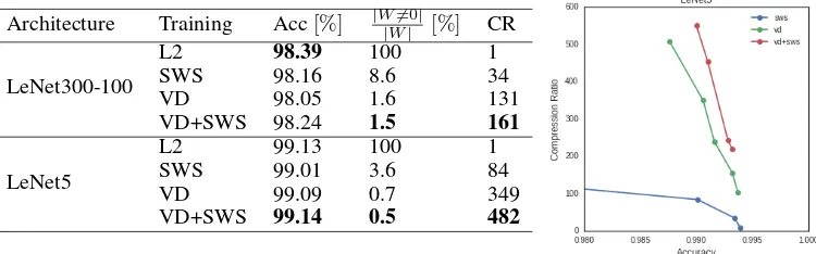
In preliminary experiments, we compare the compression ratio as proposed by Han et al. [2015] and accuracy achieved by different Bayesian compression techniques on the well studied MNIST dataset with dense (LeNet300-100) and convolutional (LeNet5) architectures. The details of the training procedure are described in appendix A.
The preliminary results presented in table 2 suggests that the joint procedure presented in this paper results in a dramatic increase of the compression ratio, achieving state-of-the-art results for both the dense and convolutional network architectures. Further work could address the interaction between the soft-weight sharing methodology and structured sparsity inducing techniques [Wen et al., 2016, Louizos et al., 2017] to reduce the overhead introduced by the compression format.
Table 2:Test accuracy (Acc), percentage of non-zero weights and compression ratio (CR) evaluated on the MNIST classification task.Soft-weight sharing(SWS) [Ullrich et al., 2017] and theVariational Dropout(VD) [Molchanov et al., 2017] approaches are compared with the Ridge regression (L2) and the combined approach proposed in this work (VD+SWS). All the accuracies are evaluated on the compressed models (details on the compression scheme in appendix B). The figure reports the best accuracies and compression ratios obtained by the three different techniques on the LeNet5 architecture by changing the values of the hyper-parameters.
Architecture Training Acc[%] |W|W6=0||[%] CR
LeNet300-100
L2 98.39 100 1
References
K. Ullrich, E. Meeds, and M. Welling. Soft Weight-Sharing for Neural Network Compression.ICLR, 2017.
Steven J. Nowlan and Geoffrey E. Hinton. Simplifying neural networks by soft weight-sharing. Neural Comput., 4(4):473–493, July 1992. ISSN 0899-7667. doi: 10.1162/neco.1992.4.4.473. URLhttp://dx.doi.org/10.1162/neco.1992.4.4.473.
D. Molchanov, A. Ashukha, and D. Vetrov. Variational Dropout Sparsifies Deep Neural Networks. ICML, January 2017.
D. P. Kingma, T. Salimans, and M. Welling. Variational Dropout and the Local Reparameterization Trick.ArXiv e-prints, June 2015.
S. Han, H. Mao, and W. J. Dally. Deep Compression: Compressing Deep Neural Networks with Pruning, Trained Quantization and Huffman Coding.ArXiv e-prints, October 2015.
Wei Wen, Chunpeng Wu, Yandan Wang, Yiran Chen, and Hai Li. Learning structured sparsity in deep neural networks. CoRR, abs/1608.03665, 2016. URLhttp://arxiv.org/abs/1608.03665. Christos Louizos, Karen Ullrich, and Max Welling. Bayesian compression for deep learning. NIPS,
2017.
Appendices
A
Training
The full training objective equation is given by the variational lower bound in equation 1, where the two KL-Divergence terms have been scaled according to two coefficientsτ1andτ2respectively:
L(φ,ψ) =LD(φ)−DKL(qφ(w,m)||pψ(w,m))
=LD(φ)−
D
X
i=1
τ1DKL
N wi|θi, σ2i
|| 1 |wi|
+τ2logGMψ(mi=θi)
+C
Starting from a pre-trained model, in a first warm-up phase we setτ1= 1andτ2= 0. Note that this part of the training procedure matches the Sparse Variational Dropout methodology [Molchanov et al., 2017]. After reaching convergence (200 epochs in our experiments), we initialize the parametersψ
for the mixture model and the coefficientτ2is set to a value of2 10−2(τ1is kept to1) to induce the clustering effect with the Soft Weight sharing procedure. This phase usually requires 50-100 epochs to reach convergence.
The mixture model used for our experiments uses 17 components, one of which has been fixed to zero with a fixed mixing proportionπ0= 0.999. A gamma hyper-prior (α= 105,β= 10) have been applied to the precision of the Gaussian components to ensure numerical stability.
The proposed parametrization stores the weight varianceσ2, each mixture component precision
Table 3:Learning rates and initialization values corresponding to the model parameters.wrepresents the weight vector of a pre-trained model, while∆µrepresent the distance between the means of the mixing components and it is obtained by dividing two times the standard deviation of thewdistribution by the number of mixing componentsK. Note that the indexingigoes from1toDwhilekstarts from−
K
−1
2 and reaches
K
−1 2 .
θi logσ2i µk logλk logπk
Initialization wi -10 k∆µ −2 log (0.9 ∆µ)
log 0.999 k= 0 log1−π0
K k6= 0
Learning Rate 5 10−5 10−4 10−4 10−4 3 10−3
B
Compression
The computation of the maximum compression ratio has been done accordingly to the procedure reported in Han et al. [2015]. The first part of the pipeline slightly differs according to the methodolo-gies:
1. Sparse Variational Dropout (VD)
At the end of the Sparse Variational Dropout training procedure (VD) all the parameters with a corresponding binary dropout rate greater then a fixed threshold (bi=σi2/ θi2+σi2
≥
0.95) are set to zero [Molchanov et al., 2017]. Secondly, the weight meansθare clustered with a 64-components mixture model and they are collapsed into the mean of the Gaussian with the highest responsibility.
2. Soft Weight Sharing (SWS) and joint approach (SWS+VD)
Once the training procedures involving the mixture of Gaussian model have converged to a stable configuration, the overlapping components are merged and all the weights are collapsed into the mean of the component that corresponds to the highest responsibility (see Ullrich et al. [2017] for details). Since the weight assigned to the zero-centered component are automatically set to zero, there is no need to specify a pruning threshold.
At the end of this initial phases, the models are represented as a sequence of sparse matrices containing discrete assignments. Empty columns and filters banks are removed and the model architecture is adjusted accordingly. The discrete assignments are encoded using the Huffman compression scheme and the resulting matrices are stored according to the CSC format using 5 and 8 bits to represents the offset between the entries in dense and convolutional layers respectively.
C
Derivation of the KL-Divergence
In order to compute the KL-divergence between the joint prior and approximate posterior distribution, we use the factorization reported in table 1:
−DKL(qφ(w,m)||pψ(w,m)) =
Z Z
qφ(w,m) logpψ( w,m) qφ(w,m)d
wdm
=
D
X
i=1
Z Z
qσi(wi|mi) qθi(mi) log
p(wi)pψ(mi)
qσi(wi|mi) qθi(mi)
By plugging inqθi(mi) =δθi(mi)and observing Where the first KL-divergence can be approximated according to Molchanov et al. [2017]:
DKL(qσi(wi|mi=θi)||p(wi)) =DKL
While the second term can be computed by decomposing the KL-divergence into the entropy of the approximate posteriorH(qθi(mi))and the cross-entropy between prior and posterior distributions
H(qθi(mi), pψ(mi)). Note that the entropy of a delta distribution does not depend on the parameter
θi, therefore it can be considered to be constant.
DKL(qθi(mi)||pψ(mi)) =−H(qθi(mi)) +H(qθi(mi), pψ(mi))