www.elsevier.nlrlocaterjappgeo
Mapping of subsurface karst structure with gamma ray and
electrical resistivity profiles: a case study from Pokhara valley,
central Nepal
Pitambar Gautam
),1, Surendra Raj Pant, Hisao Ando
2 Central Department of Geology, TribhuÕan UniÕersity, Kirtipur, Kathmandu, NepalReceived 3 August 1999; accepted 10 July 2000
Abstract
Ž .
Electrical resistivity sounding with Schlumberger array and dipole–dipole imaging and natural gamma ray intensity
Ž .
measurements were made over the karst features subsurface flow-channels, solution cavities, sinkholes in the Pokhara valley, central Nepal. In the Powerhouse area, the upper 60–80 m section of the basin-filling Quaternary sediments is
Ž . Ž .
represented by layered clastic sediments gravel, silt, clay that are represented by KQ-type r1-r2)r3)r4 electrical
Ž . Ž
sounding ES curves. The true electrical resistivity of the layers has a wide range of variation a few hundreds to several
.
tens of thousands ofVm such that it is possible to determine both the vertical and lateral subsurface geological variations by integrating the electrical resistivity profiling and sounding techniques. Total gamma ray intensity profiles measured over
Ž .
various karstified locations reveal significant anomalies up to 100 counts per second, cps over the known or unknown subsurface openings. In the Powerhouse area, presence of a network of at least three linear NNE–SSW oriented subsurface channels, made by past and present underground flow-channels, is inferred. In interpreted electrical image profiles, contours of elevated resistivity reflect the cross-sectional geometry of cavities. The gamma-ray method is sensitive to near-surface
Ž .
cavities while the electrical image effectively locates the void spaces at intermediate up to 5–20 m depths. An exploration program involving rapid radiometric mapping followed by selective electrical imaging is recommended for future exploration of karst-prone areas in the valley.q2000 Elsevier Science B.V. All rights reserved.
Keywords: Nepal; Pokhara valley; Karst; Electrical resistivity; Radioactivity methods; Quaternary
)Corresponding author. G.P.O. Box 9323, Kathmandu,
Nepal. Tel.:q977-1-525-648.
E-mail address: gautam@ ptugeo.wlink.com.np
ŽP. Gautam ..
1
Temporarily until end of July 2000 at: cro Prof. Dr. E. Appel, Institute of Geology and Paleontology, University of Tuebingen, Sigwartstrasse 10, 72076 Tuebingen, Ger-many. Tel.:q49-89-7071-74132.
2 Ž
Present address: Suimonchishitsu Kenkyuusho
Ins-.
titute of Hydrogeology Co. Ltd. , Sapporo 060-0004, Japan.
1. Introduction
Ž .
The Pokhara valley ca. 50 km=5 km rep-resents an intermontane fluvial basin spread around the midstream of the Seti river in the Lesser Himalaya of Nepal. It is filled by large
Ž
volume of layered clastic deposits gravel, silt
.
and clay of Quaternary age, brought from the Annapurna mountain range probably by a series
0926-9851r00r$ - see front matterq2000 Elsevier Science B.V. All rights reserved. Ž .
Ž
of catastrophic debris flows Yamanaka et al.,
.
1982 . Due to the presence of easily soluble
Ž .
calcareous material 25–65%, by volume in the clastic sediments, splendid river terraces and deep gorges are carved by the Seti river and its
Ž
tributaries. Karst structures subsurface flow-channels, solution cavities, sinkholes, pinnacles,
.
solution chimneys, etc. are widely developed both at the surface and underground. The karst structures, whether exposed or not, pose serious threat to houses, farmlands and public work of
Ž
any scale e.g., the collapse of a highway bridge
.
over the Seti river; Dhital and Giri, 1993 . This study deals with the first results of geophysical investigations of buried karst struc-tures in the Pokhara city, which is a site of construction works of various scales. Though we concentrated in three areas of known karst structures: the Powerhouse area in the south, Gupteshwar–Patale Chhango cave system in the southwest and Mahendra–Chamero cave system at Batulechaur in the north, we present here data from only the former two areas. Methods used
Ž
are: shallow electrical resistivity sounding
sym-. Ž
metrical Schlumberger , electrical imaging
di-.
pole–dipole , and radiometric gamma survey. We aimed at detection of the large-scale lateral and vertical changes in overburden lithology on
Ž
the basis of electrical resistivity Keller and
.
Frischknecht, 1966 , appraisal of the influence of the karstic features to the resistivity-depth
Ž
models at relatively small scale e.g., Ward,
.
1990 and also delineation of shallow karst features by measuring the gamma ray counts
ŽNielson et al., 1990; Sharma, 1997 , respec-.
tively. Seismic refraction and magnetometry could not be used due to strong industrial elec-tricalrelectromagnetic noise of unknown origin.
2. Geological and speleological characteristics
2.1. Brief geological outline
The Quaternary deposits that overlie the mid-land metasedimentary rocks, of Precambrian
age, forming the basement in the Pokhara valley are divisible into seven formations: Begnas, Siswa, Tallakot, Ghachok, Phewa, Pokhara and
Ž .
Rupakot Formations Yamanaka et al., 1982 . The Ghachok, Pokhara and Phewa Formations are the major lithologies prone to the
develop-Ž .
ment of the karstic features Fig. 1 . The Gha-chok Formation is represented by extremely hard conglomerate bed made up of sub-angular to sub-rounded gravels of limestone, sandstone and shale cemented by calcareous material. The Pokhara Formation is made up of fluvial gravels with intercalations of lacustrine sediments; the gravels comprise sub-angular to sub-rounded pebbles and cobbles of limestone and calcareous shale, which exhibit poor cementation, ill-sort-ing, and partial stratification. The Phewa For-mation comprises well stratified, porous and comparatively weak deposits of calcarenite to calcisiltite composition.
A notable lithological unit is the gravel ve-neer on the fillstrath terraces carved in the Pokhara Terrace. The veneer gravels are of mainly cobble to boulder size, larger than those in the Pokhara Formation, mostly sub-rounded and scattered in unsorted sandy matrix. The clasts are represented by mainly gneiss, granite, quartzite and schist. Major geomorphologic units
Ž .
are: i Ghachok Terrace and Pokhara Terrace representing the accumulational fill-top
land-Ž .
forms; ii two groups of fillstrath terraces de-veloped over the Ghachok and Pokhara Ter-races, respectively, representing landforms formed by redeposition over eroded ancient
ter-Ž . Ž
races; and iii recent flood plain Yamanaka et
.
al., 1982 .
2.2. Speleological characteristics
Ž .
Gebauer 1983 described 10 cave-sites from the western part of the Pokhara valley, of which three prominent sites of development of karst features are indicated in Fig. 1. They are: the
Ž .
Ž .
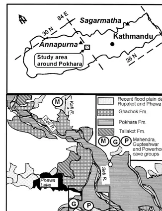
Fig. 1. Sketch map of Nepal showing the study area in Pokhara valley upper diagram and schematic geologic map with
Ž . X
major lithological units lower diagram; adapted from Yamanaka et al., 1982 . The Pokhara city lies at ;28812 N latitude and 83858X E longitude. The Phewa lake is shown in dark color. Three prominent localities of the karstic features or caves
ŽM, G and P are shown after Gebauer 1983 .. Ž .
Ž .G which comprises the Patale Chhango Devi’sŽ .
fall and Gupteshwar caves formed along the course of Marde river; and the PowerStation
Ž .
caves P which occur at the terrace scarps at
Ž
the northern bank of the Phusre river Figs. 1
.
and 2 . According to him, the PowerStation caves are developed in the caprock, composed of coarse conglomerate, of relatively greater
resistance to weathering, constituting the upper-most part of the river terrace. The Mahendra and Chamero caves are developed below the
Ž
coarse conglomerate of the caprock which
.
makes actually the ceilings of the caves . The
Ž .
Ž
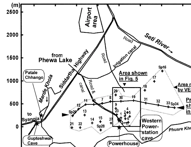
Fig. 2. The Powerhouse–Chhorepatan area. Locations of major caves stars: Patale Chhango or Devi’s Fall, Gupteshwar
.
cave, western PowerStation cave . The irregular polygon shows the area studied by ES. The stations are identified by
Ž .
numbers for clarity, only a few of them are preceded byASpB meaning sounding point .
the Indian Subcontinent. He further notes that the coarse conglomeratic caprock commonly forms the ceiling of the caves.
The Mahendra and Gupteshwar caves, which are regularly visited by tourists and therefore represent the sites prone to hazard related to possible failures of certain parts, are developed
Ž
within the Phewa Formation Koirala et al.,
.
1996 . In the Powerhouse area, subsurface flow channels or caves are developed within the con-glomerate layers that constitute the upper part of the Pokhara Formation. These layers are actu-ally overlain by a coarse gravelly conglomerate of the gravel veneers or caprocks. The floor of the caves comprises sediments represented by laminated fine sand, silt and clay, which appear gray or light brown. The main entrance to the Gupteshwar cave is located at the base of a ;4 m deep open sinkhole formed within the terrace. After entering the cave, one follows a steep course descending towards the northeast and reaches a gigantic gallery which opens up
to-wards both sides. The southern peripheries of the Powerhouse, Gupteshwar cave, Mahendra cave and Chamero cave areas have high hazard of sinkhole development, subsidence and also widespread pollution along the subsurface
solu-Ž .
tion channels Koirala et al., 1996 . The remain-ing part of the Powerhouse area was given a rating of medium hazard of sinkhole develop-ment and subsidence.
Ž .
In the Powerhouse area, Gebauer 1983 rec-ognized the western and eastern PowerStation caves located at ;15 m below the cliff from
Ž .
the top of the terrace Fig. 2 . They lie to the east of the penstock pipes: the western one at 30 m distance and the eastern one about 100 m further east. In 1982, the main passage of the western PowerStation cave was found hidden behind a large pile of pebbles; it was about 6–8 m broad and up to 5 m high resembling a
Ž .
19.2 m below the cliff top and had a nearly circular cross-section for about 5 m of the pas-sage. The passage appeared to have greater height inside, the width and height varied and followed a complex and curved course after-wards. In the eastern PowerStation cave, accord-ing to his sketches, five entrances lead into the terrace cliff from ;100 m long overhang. The three westernmost entrances rejoin in a 50 m long hall developed parallel to the terrace cliff.
3. Geophysical investigations
3.1. Field obserÕations
Geoelectrical investigations included sound-ing and imagsound-ing techniques. The equipment used
Ž
comprised: SAS 300-C Terrameter ABEM,
. Ž .
Sweden for imaging and DDR-2 IGIS, India resistivity meter for sounding studies. For
elec-Ž .
trical sounding ES with Schlumbergr array,
Ž .
the maximum current electrode separation AB was limited to 100–120 m because of strong and random industrial electromagnetic noise that was induced in the cables of electrodes spaced at larger distances. For electrical imaging, a double-dipole array comprising in-line current
Ž .
electrodes transmitter pair and potential
elec-Ž .
trodes receiver pair was used. The distance between the nearest electrodes of the transmitter
Ž .
and receiver pairs was varied as a multiple na of the electrode spacing a in each pair. Mea-surements were made at several discrete posi-tions as the receiver pair was moved incremen-tally away from the fixed transmitter pair to a maximum distance given by ns10. The trans-mitter pair was then moved by one increment
Ž .a along the profile and the procedure was repeated. These measurements aimed at obtain-ing a continuous 2D coverage of the subsurface, as a combination of lateral profiling and vertical
Ž .
sounding Telford et al., 1990 along selected profiles. The ES stations are within the irregular polygon, whereas several dipole–dipole array profiles were taken in the Powerhouse and
Ž
Gupteshwar cave–Patale Chhango areas see
.
Figs. 2 and 5 .
A GRS-500 portable differential gamma-ray
Ž .
spectrometer Scintrex, Canada equipped with
Ž .
124 cc NaI Tl detector was used to measure the
Ž
response mainly in Tc1 energy window total gamma-ray counts with gamma-ray energy Eg
.
)0.08 MeV; recording periods10 s . The area mapped by gamma ray method lies within the uppermost river terrace, at the northern bank of Phusre river, shown in Figs. 2 and 5. Gamma-ray
Ž
intensity was measured at two levels on the daylight surface or the topsoil and in air at waist
.
height with a spacing of 5 or 2.5 m along two profiles. These measurements were taken after the observations taken over the Mahendra cave where elevated gamma-ray readings were found directly over the depressions, of various scales, caused by collapsersubsidence of the ground. It was found that significant variations occur at both observation levels. The readings taken at the soil surface were higher but erratic com-pared to the readings taken at waste height. The latter type of measurement was preferred for mass measurement because it was almost equally informative as the former but clearly faster.
Ž .
A conductivity-meter Yokogawa, Japan was used to measure the electrical conductivity of water samples from different rivers, lake and springs or caves.
3.2. Interpretation techniques
Preliminary estimation of the layer
parame-Ž .
ters resistivity and thickness from an ES curve was attempted by matching it with two-layer master and auxiliary curves. The layer parame-ters were later used as initial estimates for fur-ther processing by iterative 1D inversion code which combines the linear filtering and ridge regression techniques to obtain best-fit models
Ž
in the least square sense Inman, 1975;
Koe-.
foed, 1979 .
value is related to the center point of the spread along the profile and the particular n-value along the vertical. Pseudosections were generated by contouring data recalculated along regular grids by triangulationrlinear interpolation. Inversion of the pseudosections was done using RES2DINV software which works on the smoothness-constrained least-square method with implementation of quasi-Newton
optimiza-Ž .
tion technique Loke and Barker, 1996 . The inversion program uses a 2D model in which the subsurface consists of an arrangement of blocks forming a layered rectangular mesh in the vertical plane. The program automatically determines the distribution of the blocks and their size so that the number of blocks does not exceed the number of datum points. For the dipole–dipole array, the thickness of the upper-most layer is set to 0.3 times the electrode spacing. The thickness of each subsequent lay-ers is increased by 10% or 25%. The output of the inversion is in the form of resistivity-depth model consisting of an arrangement of rectangu-lar blocks with true resistivity values loosely tied to the distribution of datum points in the pseudosection and a calculated apparent resistiv-ity section. The depth of the bottom row of blocks in the model is set to be approximately
Ž .
equal to the depth of investigation DOI appli-cable for the maximum size of the array
ob-Ž .
tained after Edwards 1977 .
Additionally, interpretation was attempted also with another 2D-inversion software that utilizes the concept of the sensitivity
coeffi-Ž
cients for the underlying theory, see Dietrich,
. Ž
1999 . According to Dietrich P. Dietrich, Uni-versity of Tubingen, personal communication,
¨
.
2000 , the DOI is regarded as a function of a specified deviation in electrical conductivity, an assumed area of deviation and a measured impedance contrast. The 2D model used in the inversion consists of an arrangement of blocks forming a layered rectangular mesh as in the RES2DINV software with a difference that the blocks in this case are of equal size. The pro-gram assigns an initial resistivity value to each
node forming the mesh and assumes smooth variation of resistivity between the nodes. This inversion scheme generates a model section that has much larger area than that represented in the corresponding pseudosection.
For all 1D and 2D inversion data presented in this paper, the quality of the fit between the pair
Ž .
of m data-points is1,2,3 . . . , m of observed
Ž .
apparent resistivity robs and calculated
appar-Ž .
ent resistivity rcal for the accepted model is given by a parameter called percent RMS error
Ž´RMS.. It is calculated as follows
Analysis of radiometric data was carried out initially along individual profiles. A contour map was generated by gridding the dataset from adjacent profiles to correlate the visual anoma-lous features.
3.3. Results of inÕestigations
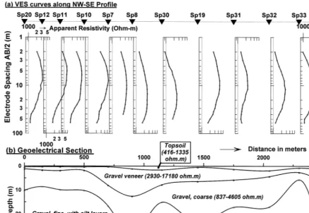
3.3.1. LithologicalÕariations by ES data Fig. 3 illustrates the typical ES curve recorded in the study area and the interpretation made to obtain estimates of the layer parameters. The equivalent models presented are those for which forward solution using the corresponding layer parameters yield curves which fit the observed values within an arbitrarily assigned ´RMS of 10%. A summary of the layer parameters is presented in Table 1. Consideration of the layer parameters obtained for the best-fitting models to ES curves for 34 stations suggests the pres-ence of significant lithological variability in the uppermost part of the basin-filling deposits. In general, the subsurface medium comprises a
Ž .
four-layer structure as follows: a a topmost
Ž
soil layer with varying moisture content r1s
. Ž .
Fig. 3. Bilogarithmic plots showing a typical electrical
Ž .
sounding Schlumberger array curve and its interpretation in terms of layered models. Both the apparent resistivity
Žfor measured and fitted curves and true resistivity for. Ž .
the models share the same horizontal axis; the electrode
Ž .
spacing ABr2 and depths to the different layers share
Ž .
the same vertical axis. The RMS error ´RMS for the best-fitting curve is 3.8% while it has a maximum value of 10% for the equivalent models shown. The layer parame-ters are listed in Table 1.
cobbles, boulders and pebbles in a sandy matrix
Žr2s2131–25698 V m; h2s0.7–11.43 m ;. Ž .c the third layer of gravel, of intermediate
Ž
resistivity and extremely varying thickness r3
.
s495–8728 V m; h3s0.64–37 m , probably
Ž
with greater amount of finer material sand and
.
clay , low degree of cementation and relatively
Ž .
high moisture content; and d the fourth layer comprising silt and clay of lowest resistivity
Žr4s13–1793 V m . The latter two layers.
belong to the Pokhara Formation.
Despite the possible uncertainties in ranges of the suggested layer parameters due to the principle of equivalence, the actual observations prove the general validity of the interpreted layer parameters. Such a four-layer sequence is exposed in a cliff near the eastern PowerStation
Ž .
cave where one observes: a topsoil layer,
sev-Ž .
eral cm thick; b compact and coarse gravel
Ž .
down to 5 m; c gravel with occasional lenses
Ž .
of silt down to 17.2 m; and d silt with clay intercalations further below. Also, it may be noted that the second and third layer may not be very well differentiated in some curves.
Fig. 4 shows the geoelectrical section based on data from ES stations located along a NW– SE profile. The ranges of true resistivity as-signed to the layers are those obtained from models which best fit the observed curves used to construct this particular profile. It clearly illustrates the subsurface lithological variations. A noteworthy observation is the gradual change in the depth of the base of the gravel veneer and the third layer from both sides toward the cen-ter. The depth is maximum below Sp8, which probably represents the center of the debris fan
Žin Fig. 4 ..
Table 1
Ž .
Summary of layer parameters based on interpretation of a typical sounding curve Sp2
Layer no. Parameters for the best-fitting model Limits for equivalent models
Žwith 3.8% RMS error. Žwith up to 10% RMS error.
Resistivity Thickness Longitudinal Transverse Resistivity Thickness
ŽVm. Ž .m conductance resistance ŽVm. Ž .m
2
ŽmS. ŽVm . Min. Max. Min. Max.
1 1451 1.96 1360 2855 1303 1622 1.44 2.72
2 3930 6.41 1630 25201 3221 4835 4.33 9.55
3 2008 10.07 5010 20222 1071 3079 4.89 28.27
Ž .
Fig. 4. The electrical sounding with Schlumberger array curves and the interpreted geoelectrical section along a NW–SE
Ž .
profile see Fig. 2 for location .
3.3.2. Delineation of subsurface flow-channels by gamma-ray counts
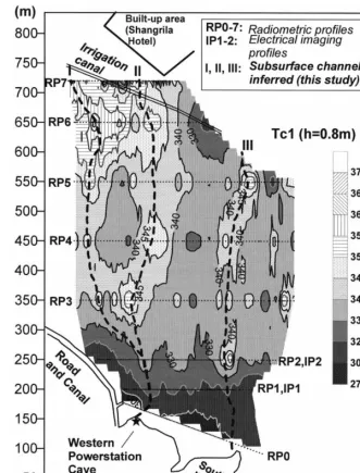
A contour map of total gamma ray counts derived from eight profiles is shown in Fig. 5. The interpretation of gamma-ray counts in terms of the subsurface lithology or mass distribution is not straightforward for many reasons. The total radiation measured also involves cosmic radiation; only a fraction representing the rela-tive differences is due to variation in local radioactivity emissions. The measured gamma-ray activity in the field is a sum of the back-ground of the measuring instrument, intensity of cosmic rays, radioactivity of the constituent near surface rock or soil medium, effect of possible
Ž
radioactive fallout, and the radon primarily
222.
Rn content in the air. The latter is known to
fluctuate with the variations in temperature, hu-midity and pressure, which affect the escape of radon from the rock or soil medium. With fa-vorable circulation of radon and mineralized groundwater, the fracture and fault zones are enriched with the decay products of Ra and Rn and may be the sites of redistribution of K40,
U238 and Th236. Despite these uncertainties, the areas lying above the karst structures are known to possess increased gamma activity due to the increased propagation of the emission along the
Ž
fissures or fractures to the surface Surbeck and Medici, 1990; Abdoh and Pilkington, 1989; and
.
Fig. 5. Contour map of total gamma ray counts recorded by a gamma-ray spectrometer in area lying between Powerhouse
Ž .
and Shangrila Hotel area. For location see Fig. 2. RP0–RP7: radiometric profiles; IP1–IP2: imaging resistivity profiles. Discontinuous lines show the inferred traces of three subsurface channels marked by anomalous counts in the map.
scales, caused by collapsersubsidence of the ground along several radiometric profiles pass-ing over the Mahendra and Chamero caves.
From the reasons stated above, the elevated readings are attributed to the presence of
sub-Ž .
surface channels in the study area Fig. 5 . At least three subparallel channels are inferred. The
Ž .
channels which have served as pathways for drainage of water entering from the Phewa lake
Žto the NW and. ror the Seti river NE . TheŽ .
positive linear, subparallel to each other, anoma-lies resemble the radon anomaanoma-lies observed over fracture zones associated with a known fault by
Ž .
Abdoh and Pilkington 1989 . The exact mecha-nism giving rise to the anomalies in the study
Ž
area requires further investigations e.g., de-tailed differential gamma-ray spectrometer sur-vey, determination of radon concentrations in soil samples, mapping of the distribution of clay
40.
which could be source of K .
3.3.3. Electrical imaging and resistiÕity-depth
models
3.3.3.1. Powerhouse area. Fig. 6a shows the
pseudosection based on data along profile IP1 with as5 m and n-value of 1–10. For such a spread, the maximum DOI is ;13.6 m
follow-Ž .
ing Edwards 1977 but only ;10.8 m
follow-Ž .
ing Roy and Apparao 1971 . A comparison between the results of inversion shown in Fig. 6b and c with those in Fig. 6d and e reveals that the model sections have common features in terms of resistivity distribution though there is considerable difference in the depth distribution. Assuming that the elevated resistivity regions
Žsay r)5000 V m reflect the subsurface karst.
features and the depths of distribution of such features are closer to those observed at the exposed cliffs as discussed in Section 2.2 above, the model in Fig. 6e bears considerable likeness to the real situation. The differences in depth distribution may stem from the way the concept of DOI is considered during inversion,
non-uniqueness of the inverse problem and the devi-ations of the real situation from the adapted
Ž
2D-inversion model, etc. e.g., Barker, 1989;
.
Ward, 1990; Oldenburg and Li, 1999 .
3.3.3.2. Gupteshwar caÕe. Pseudosections con-structed from the observed and calculated ap-parent resistivities as well as the model section obtained by RES2DINV for profile over this cave are presented in Fig. 7. As this profile has a spacing of 2.5 m, which is half of that for IP1, the corresponding maximum DOI estimates also
Ž
will be half i.e., 6.8 m after Edwards, 1977 but
.
only ;5.4 m after Roy and Apparao, 1971 . The model shows the presence of essentially two sub-horizontal layers: a high resistivity gravelly layer which serves as the medium of the development of localized near surface cavi-ties and the underlying low resistivity layer consistent with the siltyrclayey lithology of the Phewa Formation. The entrance to Gupteshwar cave described in Section 2.2 lies at ;10 m to the northwest from the center of profile ID2. Lack of high resistivity regions in the lower part of the model section suggests that the main gallery of the cave lies at depths greater than those covered by the maximum DOI of the used array.
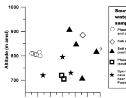
3.4. Electrical conductiÕity of water samples
Fig. 8 shows the plot of electrical
conductiv-Ž
ity of water samples from various sources from north to south they are: Kali river, Phewa lake and canal originating from it, Seti river, cave
.
and springs near Powerhouse, and Phusre river and come from several localities, whose
eleva-Ž
Fig. 6. Results of electrical imaging by dipole–dipole array along profile IP1 from the Powerhouse area see Figs. 2 and 5
. Ž . Ž . Ž . Ž .
for profile location . a Measured data; b – c results of 2D-inversion following the scheme of Loke and Barker 1996 ;
Ž . Ž . Ž .
and d – e results of 2D-inversion after Dietrich 1999 . Though the models show similar shapes, the depth distribution of
Ž .
objects of contrasting resistivity differs significantly. Model section c is the best mathematical solution as it has low´RMS.
Ž .
Ž .
Fig. 7. Results of electrical imaging by dipole–dipole array along profile ID2 over the Gupteshwar cave. a Measured data;
Ž . Ž . Ž .
and b – c results of 2D-inversion following the scheme of Loke and Barker 1996 . The model section suggests the presence of at least 6–7 m thick two-layer subsurface structure over the Gupteshwar cave.
tions are identified. The conductivity of the water samples collected from the spring or cave water is in between the conductivity range of those from Phewa lake and the Seti river. Hence, it is most likely that the water draining through
Ž .
Fig. 8. A plot of the electrical conductivity EC vs. altitude for water samples from various sources within the
Ž .
Pokhara basin. The temperature source of the water
Ž
samples were as follows: 15.5–20.08C Phewa lake and
. Ž . Ž .
canal ; 17.78C Kali river ; 12.2–18.38C Seti river ; 18.7–
Ž . Ž
19.38C Phusre river ; and 16.6–23.18C spring or cave
.
water . The spring water sample plotting at the left side
Žfrom east of the PowerStation , with lowest conductivity.
is believed to originate from the Phewa lake. The other two springrcave water samples plotting in the right side seem to have large influence of the Seti river water. A high EC value recorded from the Seti river at 820 m altitude is difficult to explain and is marked with a question mark.
a network of subparallel subsurface channels which are fed from the Seti river as well as the Phewa lake and canals.
4. Conclusions
The layered lithological structure of the Qua-ternary sediments filling the Pokhara basin can be mapped efficiently by the electrical resistiv-ity sounding technique. Gamma-ray intensresistiv-ity profiles taken over known cave areas show the presence of positive anomalies when there are karstic features in the subsurface. Areal gamma-ray mapping of the Powerhouse area reveals linear anomalous zones which are related to subsurface channels. Model sections obtained from inversion of the electrical imaging profiles in the Powerhouse and Gupteshwar cave areas reveal localized high resistivity features at-tributable to the karstic features and layered subsurface structure, respectively. In the
ab-sence of independent data on the subsurface geology based on drilling or detailed subsurface observations even in known karst areas, it is difficult at this stage to make accurate estimates of the depth of distribution of the karstic fea-tures due to the possible non-uniqueness of the inverse geophysical problem. However, a geo-physical complex involving radiometric map-ping and electrical imaging seems effective in assessing the degree of development of karst features in the subsurface medium in qualitative terms.
Acknowledgements
Dr. P.C. Adhikary, Head of the Central De-partment of Geology, Tribhuvan University
ŽCDG TU and graduate students D. Bhattarai,.
H. Gurung and R.N. Wagle supported us in organization of the field work and data acquisi-tion. The Kathmandu Office of Japan Interna-tional Cooperation Agency and CDG TU funded the fieldwork through a collaborative program. The manuscript benefitted from the discussions with P. Dietrich, information on shareware pro-vided by M.H. Loke and the critical comments of R. Guerin, N.B. Christensen and another
´
anonymous reviewer. A JSPS invited fellowship to PG for research stay at Hokkaido University provided the opportunity to compile this paper. We express our gratitude and appreciation to all persons and institutions involved.References
Abdoh, A., Pilkington, M., 1989. Radon emanation studies of the Ile Bizard Fault, Montreal. Geoexploration 25, 341–354.
Barker, R.D., 1989. Depth of investigation of collinear
Ž .
symmetrical four-electrode arrays. Geophysics 54 8 , 1031–1037.
Dhital, M.R., Giri, S., 1993. Engineering-geological inves-tigations at the collapsed Seti Bridge site, Pokhara.
Ž .
Bull. Dep. Geol., Tribhuvan Univ. 3 1 , 119–141. Dietrich, P., 1999. Konzeption und auswertung
Ž
von sensitivitatskoeffiziententen in German with En-¨
glish abstract; English title: Conception and interpreta-tion of DC-geoelectrical tracer experiments using
sensi-.
tivity coefficients . Doctoral Thesis, Univ. of Tubingen,¨
Ž .
Tubinger Geowissen-Schaftliche Arbeiten TGA C50,¨
130 pp.
Edwards, L.S., 1977. A modified pseudosection for
resis-Ž .
tivity and IP. Geophysics 42 5 , 1020–1036.
Gebauer, D.H., 1983. Caves of India and Nepal. Spelalogische Sud-Asien Expedition 1981r82, Ger-¨
many. 166 pp.
Inman, T.R., 1975. Resistivity inversion with ridge regres-sion. Geophysics 40, 798–817.
Keller, G.V., Frischknecht, F.C., 1966. Electrical Methods in Geophysical Prospecting. Pergamon Press, 519 pp. Koefoed, O., 1979. Geosounding Principles. 1: Resistivity
Sounding Measurements. Elsevier, Amsterdam, 276 pp. Koirala, A., Rimal, L.N., Sikrikar, S.M., Pradhananga, U.B., 1996. Engineering and environmental geological map of Pokhara valley. Published by Department of
Ž
Mines and Geology in cooperation with BGR,
Ger-.
many , Lainchaur, Kathmandu, Nepal.
Loke, M.H., Barker, R.D., 1996. Rapid least-squares inver-sion of apparent resistivity pseudosections by a quasi-Newton method. Geophys. Prospect. 44, 131–152.
Nielson, D.L., Linpei, C., Ward, S.H., 1990. Gamma-ray spectrometry and radon emanometry in environmental geophysics. Geotechnical and Environmental
Geo-Ž .
physics. In: Ward, S.H. Ed. , Soc. Exp. Geophys., Tulsa vol. 1, pp. 219–251.
Oldenburg, D.W., Li, Y., 1999. Estimating depth of inves-tigation in dc resistivity and IP surveys. Geophysics 64
Ž .2 , 403–416.
Roy, A., Apparao, A., 1971. Depth of investigation in
Ž .
direct current methods. Geophysics 36 5 , 943–959. Sharma, P.V., 1997. Environmental and Engineering
Geo-physics. Cambridge Univ. Press, 475 pp.
Surbeck, H., Medici, F., 1990. Rn-222 transport from soil to karst caves by percolating water, Proc. 22nd Congr., IAH, Aug. 27–Sept. 1, Lausanne. .
Telford, W.M., Geldart, L.P., Sheriff, R.E., 1990. Applied Geophysics. Cambridge Univ. Press, 770 pp.
Ward, S.H., 1990. Resistivity and induced polarization methods. Geotechnical and Environmental Geophysics.
Ž .
In: Ward, S.H. Ed. , Soc. Exp. Geophys., Tulsa vol. 1, pp. 147–189.