MEASURING AND OPTIMIZING MARKET RISK USING VINE COPULA SIMULATION.

vii

CONTENTS

 

FOREWORDS ‐‐‐‐‐‐‐‐‐‐‐‐‐‐‐‐‐‐‐‐‐‐‐‐‐‐‐‐‐‐‐‐‐‐‐‐‐‐‐‐‐‐‐‐‐‐‐‐‐‐‐‐‐‐‐‐‐‐‐‐‐‐‐‐‐‐‐‐‐‐‐‐‐‐‐‐‐‐‐‐ i 

President of the Indonesian Mathematical Society (IndoMS) ‐‐‐‐‐‐‐‐‐‐‐‐‐‐‐‐‐‐‐‐‐‐‐‐‐‐‐‐‐‐‐‐‐‐‐‐‐ ii  Chair of the Committee IICMA 2013‐‐‐‐‐‐‐‐‐‐‐‐‐‐‐‐‐‐‐‐‐‐‐‐‐‐‐‐‐‐‐‐‐‐‐‐‐‐‐‐‐‐‐‐‐‐‐‐‐‐‐‐‐‐‐‐‐‐‐‐‐‐‐‐‐‐‐ iv  INVESTIGATION OF CONSTRAINED BAYESIAN METHODS OF HYPOTHESES  TESTING WITH RESPECT TO CLASSICAL METODS 

Kartlos Joseph Kachiashvili ……….4  MATHEMATICS EDUCATION IN SINGAPORE – AN INSIDER’S PERSPECTIVE 

BERINDERJEET KAUR  ………..8  MODELING, SIMULATION ANDOPTIMIZATION: EMPLOYING MATHEMATICSIN  PRACTICE 

Martin Groetschel ……….10  STRONG AND WEAK TYPE INEQUALITIES FOR FRACTIONAL INTEGRAL 

OPERATORS ON GENERALIZED MORREY SPACES 

Hendra Gunawan ………11  THE ENDLESS LONG‐TERM PROGRAMS OF TEACHER PROFESSIONAL 

DEVELOPMENT FOR ENHANCING STUDENT’S ACHIEVEMENT IN  MATHEMATICS 

Yaya S Kusumah ……….……….12  DIGRAPH CONSTRUCTION TECHNIQUES AND THEIR CLASSIFICATIONS 

Slamin ……….13 

AN APPLICATION OF ARIMA TECHNIQUE IN DETERMINING THE RAINFALL  PREDICTION MODELS OVER SEVERAL REGIONS IN INDONESIA 

EDDY HERMAWAN1 _{AND RENDRA EDWUARD}2 _{……….………15} 

MAC WILLIAMS THEOREM FOR POSET WEIGHTS 

Aleams Barra1_{, Heide Gluesing}‐_Luerssen2 _……….17  PARALEL SESSIONS 

ON FINITE MONOTHETIC DISCRETE TOPOLOGICAL GROUPS OF PONTRYAGIN  DUALITY 

L.F.D. Bali1_, Tulus2_{, Mardiningsih}3 _{………..18} 

LINEAR INDEPENDENCE OVER THE SYMMETRIZED MAX PLUS ALGEBRA 

Gregoria Ariyanti1_{, Ari Suparwanto}2_{, and Budi Surodjo} 2 _………25 

viii

Sutopo1_{, Indah Emilia Wijayanti}2_{, sri wahyuni}3 _……….33 

REGRESSION MODEL FOR SURFACE ENERGY MINIMIZATION BASED ON  CHARACTERIZATION OF  FRACTIONAL DERIVATIVE ORDER 

Endang Rusyaman1_{,  ema carnia}2_{, Kankan Parmikanti}3_{, ……… 37} 

COMPARISON OF SENSITIVITY ANALYSIS ON LINEAR OPTIMIZATION  USING  OPTIMAL PARTITION AND OPTIMAL BASIS (IN THE SIMPLEX METHOD) AT  SOME CASES 

1 _{Bib Paruhum Silalahi,} 2 _{Mirna Sari Dewi ……….……82} 

APPLICATION OF OPTIMAL CONTROL FOR A BILINEAR STOCHASTIC MODEL IN  CELL CYCLE CANCER CHEMOTHERAPY 

D. Handayani1_{, R. Saragih} 2_{, J. Naiborhu} 3_{, N. Nuraini} 4_{………...91} 

FUNCTIONS USING PARTIAL BACKORDER 

ELIS RATNA WULAN1_{, VENESA ANDYAN}2 _………146 

A GOAL PROGRAMMING APPROACH TO SOLVE VEHICLE ROUTING  PROBLEM USING LINGO 

ATMINI DHORURI1_{, EMINUGROHO RATNA SARI}2_{, AND DWI LESTARI}3 _{………..155} 

CLUSTERING SPATIAL DATA USING AGRID+ 

Arief fatchul huda1_{, adib pratama}2 _{……….162} 

CHAOS‐BASED ENCRYPTION ALGORITHM FOR DIGITAL IMAGE 

eva nurpeti1_{, suryadi mt}2 _………169 

ix

rb. fajriya hakim ………178  ITERATIVE UPWIND FINITE DIFFERENCE METHOD WITH COMPLETED 

RICHARDSON EXTRAPOLATION FOR STATE‐CONSTRAINED OPTIMAL CONTROL  PROBLEM 

Fitri Alyani, Fery Firmansah, Wed Giyarti,Kiki A.Sugeng ………..225  CONSTRUCTION OF  , ‐VERTEX‐ANTIMAGIC TOTAL LABELINGS OF UNION  OF TADPOLE GRAPHS 

PUSPITA TYAS AGNESTI, DENNY RIAMA SILABAN, KIKI ARIYANTI SUGENG ………231  SUPER ANTIMAGICNESS OF TRIANGULAR BOOK AND DIAMON LADDER  GRAPHS 

Dafik1_, Slamin2_{, Fitriana Eka R}3_{, Laelatus Sya’diyah}4 _{………..………237} 

STUDENT ENGAGEMENT MODEL OF MATHEMATICS DEPARTMENT’S  STUDENTS OF UNIVERSITY OF INDONESIA 

1st_{rianti setiadi}1 _{……….…245} 

DESIGNING ADDITION OPERATION  LEARNING IN THE MATHEMATICS OF  GASING FOR RURAL AREA STUDENT IN INDONESIA 

EARLY DRUGS DETECTION TENDENCY FACTOR’S MODEL OF FRESH STUDENTS  IN MATHEMATICS DEPARTMENT UI 

DIAN NURLITA1_{, RIANTI SETIADI}2 _{……….287} 

COMPARISON OF LOGIT MODEL AND PROBIT MODEL ON MULTIVARIATE  BINARY RESPONSE 

JAKA NUGRAHA ………294  MULTISTATE HIDDEN MARKOV MODEL FOR HEALTH INSURANCE PREMIUM  CALCULATION 

x

THEORETICAL METODOLOGY STUDY BETWEEN MSPC VARIABLE REDUCTION  AND AXIOMATIC DESIGN 

Sri Enny Triwidiastuti  ………314  AN APPLICATION OF ARIMA TECHNIQUE IN DETERMINING THE RAINFALL  PREDICTION MODELS OVER SEVERAL REGIONS IN INDONESIA  

Proceeding of IICMA 2013 Mathematics Finance

265

MEASURING AND OPTIMIZING MARKET RISK USING

VINE COPULA SIMULATION

K

τMAσG

D

HARMAWAσ 1

1_{Department of Mathematics, Udayana University}

E-mail: dhramawan.komang@gmail.com

Abstract. Copula models have increasingly become popular for the modeling of the dependence structure of financial risks. The most recent copula topic is vine copula or pair copula construction (PCC). This paper is concerned with the application of pair-copula construction for measuring and optimizing the market risk of a portfolio. The dependence among the assets is modeled using a copula based on pair-copula constructions or known as vine copula, C-vine and D-vine. Furthermore, a pairwise copula model is also discussed in this paper. In order to achieve this aim, the return of each stock price is characterized individually. The main objective of this paper is firstly to show how PCC may be useful measuring and modeling market risk. The paper are also combining important results published recently. Secondly, to show PCC can be used to model the tail dependence of log-return distribution. Thirdly, to show the uses of stepwise semiparametric estimators for the estimations of market risk in multivariate log-return data. Fourthly, to show how PCC may be used on a daily basis in finance, in particular for constructing efficient frontiers and computing Conditional VaR. The paper is also to verify whether and how the optimal portfolio composition discussed may change utilizing various types of copula families and their construction, such as pairwise or vine. To do this, four Indonesian Blue Chip stocksμ ASSI=Astra International Tbk, BMRI=Bank Mandiri (Persero) Tbk., PTBA=Tambang Batubara Bukit Asam Tbk., IσTP=Indocement Tunggal Perkasa Tbk recorded during the period of 6-11-2006 to 2-08-2013 are used to compose the stock portfolio. The VaR and Conditional VaR of the stock portfolio is minimized by various types of copula and their pair constructions. The use of stepwise semiparametric estimation is also demonstrated in this paper.

Key words and Phrasesμ Value at Risk, Conditional Valur at Risk, Vine Copula, multivariate copula

1. Introduction

266

(PCC) is further developed by Bedford and Cooke [4, 5], [8] and Kurowicka and Cooke [11]. Aas et al. [1] have given the inferential methodology of how to infer the parameters available in PCC. This inferential method has stimulated the use of the PCC in various applications (see, for example, Schepsmeier et al. [20], σikoloulopoulos et al. [18], Min and Czado [14], and Mendes et al. [12]. There have also been some recent applications of copulas in the context of time series models (see the survey by Patton [19] and the recently developed CτPAR model of Brechmann and Czado [7], which provides a vector autoregressive VAR model for analyzing the non-linear and asymmetric co-dependencies between two series).

This paper emphasizes the uses of vine copulae as they are useful tools to be implemented efficiently in simulating the multivariate distribution. In fact, copula functions can be used to model the dependence structure independently of the marginal distributions. By this method, a multi-variate distribution with different margins and a dependence structure can be constructed. This paper is intended to provide some applications of pair copula constructions in portfolio risk computations and efficient frontiers. The estimation of the parameters is based on the maximum likelihood method given by Vogiatzoglou [23].

Furthermore, this paper also applies the supplement (or alternative) to VaR, that is the Conditional Value-at-Risk. The CVaR risk measure is closely related to VaR. For continuous distributions, CVaR is defined as the conditional expected loss under the condition that it exceeds VaR, see Rockafellar and Uryasev [21, 22]. For continuous distributions, this risk measure also is known as Mean Excess Loss, Mean Shortfall, or Tail Value-at- Risk. However, for general distributions, including discrete distributions, CVaR is defined as the weighted average of VaR and losses strictly exceeding VaR. Recently, the redefinition of expected shortfall similarly to CVaR can be found in [2]. For general distributions, CVaR, which is a quite similar to VaR measure of risk has more attractive properties than VaR. CVaR is sub-additive and convex explained ([21] and [22]. Moreover, CVaR is a coherent measure of risk discussed in [3] and proved in [15].

The main objective of this paper is firstly to show how PCC may be useful measuring and modeling market risk. The paper are also combining important results published recently such as [1],[4, 5], [8], [11], [12], [14], and [18]. Secondly, to show PCC can be used to model the tail dependence of log-return distribution. Thirdly, to show the uses of stepwise semiparametric estimators for the estimations of market risk in multivariate log-return data. Fourthly, to show how PCC may be used on a daily basis in finance, in particular for constructing efficient frontiers and computing Conditional VaR.

2. Pair-Copulas Constructions: A brief review

Consider a stationary d dimensional process X = (X1,··· ,Xd). If X is a

continuous random vector with joint cumulative distribution function (c.d.f.) F with

density function f, and marginal c.d.f.s Fi with density functions fi, for i = 1,··· ,d,

then there exists a unique copula C defined on [0,1]d such that

  C(F1(x1),··· ,Fd(xd)) = F(x1,··· ,xd) (1)

holds for any (x1,...,xd)  Rd (Sklar’s theorem, Sklar (1959), σelsen [17]). Therefore

267

modeling through copulas allows for factoring the joint distribution into its marginal univariate distributions and a dependence structure, its copula. By taking partial derivatives of (1) one obtains

, … , ; , … , … , ;

for some d-dimensional copula density c1···dwith parameter θ.

This decomposition allows for estimating the marginal distributions fi

separated from the dependence structure given by the d-variate copula. In practice,

this fact simplifies both the specification of the multivariate distribution and its estimation.

The decomposition of a multivariate distribution in a cascade of pair-copulas was originally proposed by Joe [10], and later discussed in detail by Bedford and Cooke [4],[5], Kurowicka and Cooke [11] and Aas et al.[1]. Refers to their results, Equation (2) can be represented as

f(x1,··· ,xd) = fd(xd) · f(xd−1|xd) · f(xd−2|xd−1,xd)···f(x1|x2,··· ,xd). (3)

The conditional densities in (3) can be written as functions of the corresponding

copula densities. That is, for every j

f(x|v1,v2,··· ,vd) = cxvj|vj(F(x|vj),F(x|vj)),··· ,f(x|vj), (4)

where vj the d-dimensional vector v excluding the j-th component. For example

when d = 4, then the four-dimensional canonical vine (C-vine) structure is

generally expressed as

f(x1,x2,x3,x4να,θ) = f(x1να1) · f(x2να2) · f(x3να3) · f(x4να4)

·c12(F(x1),F(x2)νθ12)·c13(F(x1),F(x3)νθ13)

·c14(F(x1),F(x4)νθ14)·c23|1(F(x2|x1),F(x3|x1)νθ23|1)

.c34|1(F(x2|x1),F(x4|x1)νθ34|1)

  · c34|12(F(x3|x1,x2),F(x4|x1,x2)νθ34|12), (5)

and the D-vine structure as

f(x1,x2,x3,x4να,θ) = f(x1να1) · f(x2να2) · f(x3να1) · f(x4να1)

· c12(F(x1),F(x2)νθ12)·c23(F(x2),F(x3)νθ13)

·c34(F(x3),F(x4)νθ34)·c13|2(F(x1|x2),F(x3|x2)νθ13|2)

· c24|3(F(x2|x3),F(x4|x3)νθ24|3)

268

where α and θ are the parameters of the margins and copula, respectively. The

general form of the joint probability density function (d-dimensional pdf), f() is

Figure 1. 4-dimensional D-vine copula

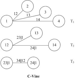
Figure 2. 4-dimensional C-vine copula

equal to

∏ , ∏ ∏ , | ,…,  

(F(xi|xi+1,··· ,xi+j−1),F(xi+1|xi+1,··· ,xi+j−1)νθ).

In a D-vine there d−1 hierarchical tress with increasing conditioning sets, and there

are d(d − 1)/2 bivariate copulas. For a detailed description, see Asa [1]. Figure 1

shows the D-vine decomposition for d = 4. It consists of 3 nested trees, where Tj

possess 5 − j nodes and 4 − j edges corresponding to pair copula. Figure 2 shows

the C-vine decomposition for d = 4. It consists of 3 nested trees, where Tj possess 5

− j nodes and 4 − j edges corresponding to pair copula.

As is mention in Berg and Aas [6] and Bedford and Cooke [4], the use of vine copula is very flexible, in this case, one may choose different copula in the bivariate.

For example, one may combine the following types of (bivariate) copulasμ

269

(lower tail) pair copula. See Joe [10] for a copula catalogue. Here below is the example D-vine consisting of Gaussian pair-copulae and margins. Parameters,

θ12,θ23,θ34, are estimated using maximum likelihood estimation method as in

Vogiatzoglou [23]. τne may refer to Haff [9] for stepwise semiparametric estimations (SSP).

  (7)

In this case, θ13,θ14, and θ24 are estimated using Kendall’s formula, that is

(8)

(9)

(10)

The following is the four dimensional C-vine consisting student’s-t margins and

Student’s t pair-copulae. Another method to calculate c23,c24 and c34 is to employ

the stepwise semiparametric (SSP) estimators developed by Haff [9]. The following example is C-Vine copula for which the parameters are estimated using SSP method.

(11)

where

270

where ui = t(xi), and t is the c.d.f. of the Students t-distribution with degrees of

freedom. See Haff [9] for d-dimensional C-vine formulation. As reported by

Vogiatzoglou in [23] that the log likelihood function of the canonical vine t-copula

model (tCVine) did not converge to a solution, hence SSP reported by Haff in [9] is alternative estimation methods. Mention in by Haff [9] that SSP estimator is computationally tractable even in high dimensions, as opposed to other methods such as MLE or IFM method.

3. Optimization of Value at Risk

Consider a portfolio consist of d stocks and denote by wi the weight of stock i

allocated to the portfolio at time t. Let f(w,r) be the loss function of the portfolio,

with w ∈ Rd is the vector of the portfolio and r is the vector of asset returns. Let

be a certain threshold, the Value-at-Risk of a portfolio at level α is defined as the

lower α−quantile of the distribution of the portfolio return

  VaR(α) = inf{ ∈ R μ P(f(w,r) ≤ ) ≥ α} (15)

The uses of VaR to measure financial risks have been increasingly popular since 1990s. VaR now becomes the standard risk measure used by financial analysts to quantify the market risk of an asset or a portfolio.

CVaR is a supplement or an alternative to VaR. CVaR is another percentile risk measure which is called Conditional Value-at-Risk. For continuous distributions, CVaR is defined as the conditional expected loss under the condition that it exceeds VaR. The following approach to CVaR is summarized from [21] and

[22]. Let rp be the return of the portfolio, then rp is defined as a random variable

satisfying rp = w1r1 + w2r2 + ··· + wdrd = wTr and the weight constrain condition is

imposed to be = 1 If the short position is not allowed then wi ≥ 0 for all t =

1,··· ,d. Let p(r) be the joint distribution of the uncertain return of the assets, the

271

∗ then is equivalent to Ψ , _,

where Ψ(w,) represents the cumulative distribution function for the associated

loss w. Assuming Ψ(w, ) is continuous with respect to , VaR(α) and CVaR(α) for

the loss f(w,r) associated with w any probability level α (0,1) can be defined by

VaR , min ∈ : Ψ , (17)

CVaR , _∈ max , , (18)

 

Equation (17) is read as the smallest value such that the probability P[f(w,r) > ]

of a loss exceeding is not larger that 1 − α. Therefore, VaRαpresents (1 − α

)-quantile of the loss distribution Ψ(w, ) and CVaRα presents the conditional

expected loss associated with w if VaRαis exceeded. Following [22], the CVaR(α)

of the loss associated with any w, it is found

  CVaR(α) = minFα(w, ), (19)

∈R

with

  r (20)

σow, the conditional value-at-risk, CVaR, is defined as the solution of an optimization problem

  r (21)

where αis the probability level such that 0 < α < 1. CVaR also is known as Mean

Excess Loss, Mean Shortfall (Expected Shortfall), or Tail Value-at-Risk, see [2]. However, for general distributions, including discrete distributions, CVaR is defined as the weighted average of VaR and losses strictly exceeding VaR, see [21]. Some properties of CVaR and VaR and their relations are studied in [2] and [15]. For general distributions, CVaR, which is a quite similar to VaR measure of risk has more attractive properties than VaR. CVaR is sub-additive and convex see [21]. Moreover, CVaR is a coherent measure of risk, proved first in [15], see also [2] and

[21].

Therefore, the problem of minimizing the Conditional Value at Risk can thus be formulated as the followingμ

  minimize r (22)

  subject to (23)

  −wT

272

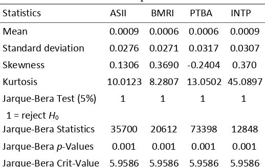
Table 1. Descriptive Statistics

Statistics  ASII  BMRI  PTBA  INTP 

Mean  0.0009 0.0006 0.0006 0.0009

Standard deviation  0.0276  0.0271  0.0317  0.0307 

Skewness  0.1306  0.3690  ‐0.2404  0.370 

Kurtosis  10.0123  8.2807  13.0502 45.0897

Jarque‐Bera Test (5%)  1  1  1  1 

1 = reject H0 

Jarque‐Bera Statistics  35700  20612  73398  12848 

Jarque‐Bera p‐Values  0.001  0.001  0.001  0.001 

Jarque‐Bera Crit‐Value  5.9586  5.9586  5.9586  5.9586 

In this case the feasibility set is X defined on region satisfying (23) and (24). Set X is convex (it is polyhedral, due to linearity in constraint (23) and (24). The optimization problem (22)-(24) are a convex programming. This problem is solved

using PortfolioCVaR class of MATLAB R2013a.

4. Empirical studies

In this section, the models of stock portfolio risk measurement and management (described in the previous sections) are implemented to a hypothetical portfolio composed by 4 Indonesian Blue Chip stocksμ ASSI=Astra International Tbk, BMRI=Bank Mandiri (Persero) Tbk., PTBA=Tambang Batubara Bukit Asam Tbk., IσTP=Indocement Tunggal Perkasa Tbk. The historical data are recorded during the period of 6 σovember 2006 to 2 August 2013. Precisely, the statistics of the 4 stocks are described in Table 1.

Table 1 reflects the mean, standard deviation, skewness, and kurtosis of the daily returns of four stocks over the period from 6 σovember 2006 to 2 August 2013. The kurtosis of all stock returns exceeds the kurtosis of normal distribution (3.0) substantially. The Jarque-Bera tests of the null hypothesis that the return distribution follow a normal distribution against the alternative that the return do not come from a normal distribution. As seen from Table 1. that the test statistics exceed the critical value at the 5% level of significant, this means that all stock returns are not normally distributed, it shows a fat tailed distribution. This means that the probability of extreme events is higher than the probability of extreme events under the normal distribution. Therefore, capturing the stock returns using normal distribution could be underestimated. When the skewness of the return data are considered, it shows that all returns are right skewed except for PTBA. This suggests that the returns are not symmetry. Again, capturing by normal distribution may result in misleading conclusions.

Using results in Table 2 and Table 3, the value of c13,c14, and c24 can be

273

Table 2. Estimated parameters and the (standard errors) from D-vine models

D‐vine copula 

stepwise semiparametric estimator (SSP) proposed by Haff [9] (Eqn.(11)-(14)), to

construct correlation matrix ρ.

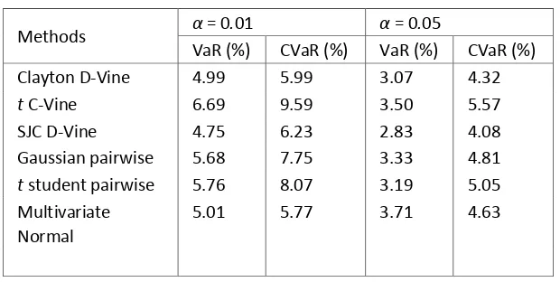
Table 4 reflects the value of VaR and CVaR simulated by Clayton D-Vine, t

C-Vine, Symmetrized Joe-Clayton (SJC) D-Vine, Gaussian pairwise, t student

274

Table 4. Simulated VaR and CVaR

Methods  α = 0.01 α = 0.05

VaR (%) CVaR (%) VaR (%) CVaR (%) 

Clayton D‐Vine  4.99 5.99 3.07 4.32 

t C‐Vine  6.69  9.59  3.50  5.57 

SJC D‐Vine  4.75 6.23 2.83 4.08 

Gaussian pairwise  5.68  7.75  3.33  4.81  t student pairwise  5.76 8.07 3.19 5.05  Multivariate 

Normal 

5.01  5.77  3.71  4.63 

         

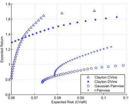
differences. The main idea of using the CVaR optimization technique is that it can reshape one tail of the loss distribution, which corresponds to high losses, and it can not account for the opposite tail representing high profits. τn the other hand, the MV approach consider the risk as the variance of the loss distribution, and since the variances (risk) can come from both tails (upper and lower), hence it is affected by high gains as well as by high losses.

5. Concluding remark

In this paper we have explored the potentials of PCC to model the dependence among financial data. A fully flexible multivariate distribution was obtained by constructing marginals with different distribution into C-vine and D-vines model. The marginals of the data show the asymmetric, high kurtosis, and

skewed right except for PTBA. The simulation results show that t-student C-vine

gives highest estimation compare with the other model (see Table 4). This is due to

the fact that the parameters of t-student C-vine model is estimated by stepwise

semiparametric estimation, which is according to Haff [9] giving higher estimates for correlations.

The pair copulas construction still needs further research on tests for choosing among copula families and among decompositions, and more powerful goodness-offit tests. Further research topics include time-varying pair-copulas may be one of interest in multivariate modeling.

275

Figure 3. Efficient frontiers simulated by pairwise and vine cop-

ula with α= 1%

References

[1] Aas, K., Czado, C., Frignessi, A. and Bakken, H. Pair-copula constructions of multiple dependence. Insuranceμ Mathematics Economics. (2009) 44μ128-198 [2] Acerbi, C., σordio, C., Sirtori, C. Expected Shortfall as a Tool for Financial Risk

Management. Working Paper, can be downloaded fromμ

httpμ//gloriamundi.com/Library Journal.asp

[3] Artzner, P., Delbaen F., Eber, J. M. and D. Heath (1999), Coherent Measures of Risk. Mathematical Finance, 9, 203-228.

[4] Bedford, T. and Cooke, R. M. Probability density decomposition for conditionally

dependent random variables modeled by vines. Annals of Mathematical and

Artificial Intelligence (2001) 32μ 245.268.

[5] Bedford, T. and Cooke, R. M. Vines: a new graphical model for dependent random variables. Ann. Statist. (2002). 30(4)μ 1031.1068.

[6] Berg, D. and Aas, K. Models for construction of higher-dimensional dependence: A comparison study. European Journal of Finance (2009), 15, 639-659.

[7] Brechmann, E.C., and C. Czado. COPAR - multivariate time-series modelling using

the COPula AutoRegressive model, Working Paper, Faculty of Mathematics,

Technical University of Munich. (2012)

[8] Cooke, R.M., H. Joe and K. Aas, Vines Arise, chapter 3 in DEPENDENCE

MODELING Vine Copula Handbook, Ed. D. Kurowicka and H. Joe, World Scienti c

Publishing Co, Singapore. (2011)

[9] Haff, I. H. Parameter estimation for pair-copula constructions. Bernoulli 19(2),

(2013), 462491

[10] Joe, H. Multivariate Models and Dependence Concepts. (1997). Londonμ Chapman

& Hall

276

[12] Mendes, B.V.d.M., Semeraro, M.M., Leal, R.P.C., Pair-copulas modeling in finance. Financial Markets and Portfolio Management (2010), 24 (2), 193-213. [13] Min, A., Czado, C., Bayesian inference for multivariate copulas using pair-copula

constructions. Journal of Financial Econometrics,(2010), 8(4).

[14] Min, A., Czado, C., Bayesian model selection for multivariate copulas using pair-copula constructions. Canadian Journal of Statistics (2011), 39(2), 239-258. [15] Pflug G. Ch. Some Remarks on the Val-ue-At-Risk and the Conditional

Value-At-Risk Inμ S. Uryasev, Ed., Pro- babilistic Constrained τptimizationμ Methodology and

Applications, Kluwer Academic Publishers, Dordrecht, (2000)

[16] MATLAB version 8.01.0 (R2013a). σatick, Massachusettsμ The MathWorks Inc., (2013).

[17] σelsen R. B. An Introduction to Copulas. Second Editions. Springer

Science+Business Media, Inc. (2006)

[18] σikoloulopoulos, A. K., Joe, H., and Li, H. . Vine copulas with asymmetric tail dependence and applications to financial return data. Computational Statistics & Data Analysis (2012), 56μ3659-3673.

[19] Patton A. J. A review of copula models for economic time series. Journal of

Multivariate Analysis 110 (2012) 418

[20] Schepsmeier U., J.Stoeber, and E.C. Brechmann. (2013). Statistical inference of vine copulasμ Vine Copula Package Version February 15, 2013. httpμ//cran.rproject.org/web/packages/VineCopula/VineCopula.pdf

[21] Rockafellar R. T. and S. Uryasev. Optimization of Conditional Value-at-Risk.

Journal of Risk, Vol. 2, (2000), pp. 21-41

[22] Rockafellar, R. T. and S. Uryasev, Conditional Value-at-Risk for General Loss Distributions, Journal of Banking and Finance (2002), Vol. 26, pp. 1443-1471. [23] Vogiatzoglou, M. Dynamic Copula Toolbox, University of Macedonia, Egnatias